Main results and figures

Overview

In this file, we provide the source code to the case studies discussed in the manuscript. For each dataset, we first empirically examine the relationship between missingness (detection) and intensity using observed data. Detection proportions are modelled by the logistic regression model fitted to the average observed intensities on the precursor-level. The design matrix is specified as the basis matrix generated on the average observed intensities with 1, 3 or 5 degrees of freedom. We show that the detection proportion is approximately linear in average observed intensity at the logit scale. To allow for missingness completely at random (MCAR) in data, we also propose a capped-logit-linear model for detection proportions where the probability of detection is capped at a value smaller than or equal to 1 for all observations in data. Lastly, the missingness mechanism is formally modelled by the detection probability curve (DPC), which describes the probability of an observation being detected given its underlying intensity. The above analyses are applied to each of the four datasets mentioned in the main text on the precursor-level. The same analyses are repeated with the four example datasets on the protein-level in the Supplementary tab of this vignette.

Load packages

library(tidyverse)
library(protDP)

Dataset A: Hybrid proteome data

Hybrid proteome samples were generated by mixing human, yeast and E.coli lysates in different ratios and analysed by SWATH-MS (Navarro et al. 2016). The original dataset (TripleTOF6600; 64-variable-window acquisition) were re-processed by DIA-NN in Demichev et al. (2020). Details of the experimental procedures and data processing steps are available in Navarro et al. (2016) and Demichev et al. (2020). The dataset was downloaded from the OSF repository at https://doi.org/10.17605/OSF.IO/6G3UX.

Data overview

We focus on the triplicates of Sample A. A log2-transformation was applied to the precursor-level intensities, before which intensity values less than 1 were already filtered out.

data("datasetA")
dat <- log2(datasetA$prec)
dim(dat)
[1] 34689     3

The dataset has a relatively small amount of missing values with an overall proportion of missing data of

sum(is.na(dat))/length(dat)
[1] 0.08632

Empirical logistic splines for detected proportions

Natural cubic splines generated on average observed intensities are fitted on detection proportions with 1, 3 and 5 degrees of freedom:

dfList <- seq(1, 5, 2)
lineColours <- RColorBrewer::brewer.pal(3, "Dark2")

nuis <- getNuisance(dat)
allFits <- list()
for (df in dfList) {
    params0 <- logitSplines_start(dp = nuis$dp, mu = nuis$mu_obs,
        wt = nuis$wt, df = df)
    fit <- logit_ztbinom(dp = nuis$dp, X = params0$X, wt = nuis$wt,
        beta0 = params0$betas_start)
    fit$binomEstimate <- params0
    allFits[[(df + 1)/2]] <- fit
    if (df == 1)
        plotEmpSplines(nuis, X = params0$X, fit$params, ylim = c(0,
            1.04), lineCol = lineColours[(df + 1)/2])
    if (df > 1)
        plotEmpSplines(nuis, X = params0$X, fit$params, ylim = c(0,
            1.04), lineCol = lineColours[(df + 1)/2], newPlot = FALSE)
}
legend("bottomright", legend = paste("df = ", dfList), col = lineColours,
    lwd = 2, lty = 1, cex = 0.8)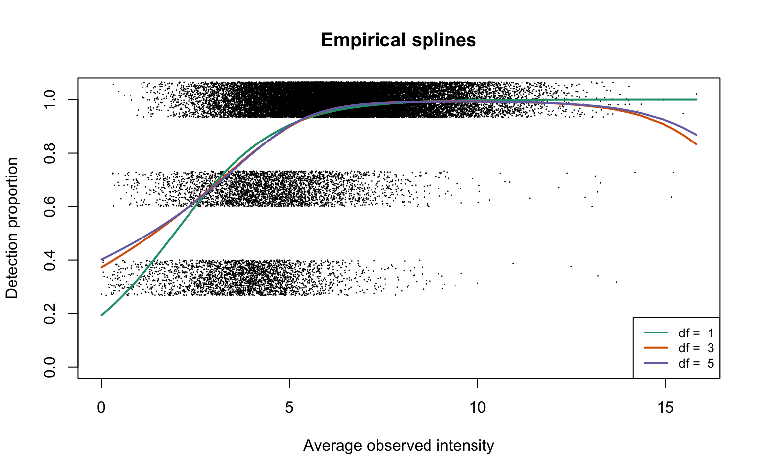

This plot corresponds to Panel (a) of Figure 1 in the manuscript.

Empirical logistic splines assuming the binomial distribution

We have assumed the number of detected samples in each precursor to follow the zero-truncated binomial distribution in the previous section. As a comparison, logistic regression splines are next fitted assuming the binomial distribution.

par(mfrow = c(1, 2))
# Plot for precursors of low intensity
low <- nuis$mu_obs < 4
nuis_low <- nuis
nuis_low$mu_obs <- nuis_low$mu_obs[low]
nuis_low$dp <- nuis_low$dp[low]
for (df in dfList) {
    params0 <- allFits[[(df + 1)/2]]$binomEstimate
    fit <- allFits[[(df + 1)/2]]
    if (df == 1)
        plotEmpSplines(nuis_low, X = params0$X[low, ], params0$betas_start,
            xlim = c(0, 4), ylim = c(-2, 2), logit = TRUE, lineCol = lineColours[(df +
                1)/2], lty = "dashed")
    plotEmpSplines(nuis_low, X = params0$X[low, ], fit$params,
        ylim = c(-2, 2), logit = TRUE, lineCol = lineColours[(df +
            1)/2], newPlot = FALSE)
    if (df > 1)
        plotEmpSplines(nuis_low, X = params0$X[low, ], params0$betas_start,
            ylim = c(-2, 2), logit = TRUE, lineCol = lineColours[(df +
                1)/2], lty = "dashed", newPlot = FALSE)
    plotEmpSplines(nuis_low, X = params0$X[low, ], fit$params,
        logit = TRUE, lineCol = lineColours[(df + 1)/2], ylim = c(-2,
            2), newPlot = FALSE)
}
legend("topleft", legend = c(paste("df = ", dfList), "Binom",
    "ZB"), col = c(lineColours, "black", "black"), lwd = 2, lty = c(1,
    1, 1, 2, 1), cex = 0.4)
for (df in dfList) {
    params0 <- allFits[[(df + 1)/2]]$binomEstimate
    fit <- allFits[[(df + 1)/2]]
    if (df == 1)
        plotEmpSplines(nuis_low, X = params0$X[low, ], params0$betas_start,
            xlim = c(0, 4), ylim = c(0, 1.04), lineCol = lineColours[(df +
                1)/2], lty = "dashed")
    plotEmpSplines(nuis_low, X = params0$X[low, ], fit$params,
        ylim = c(0, 1.04), lineCol = lineColours[(df + 1)/2],
        newPlot = FALSE)
    if (df > 1)
        plotEmpSplines(nuis_low, X = params0$X[low, ], params0$betas_start,
            ylim = c(0, 1.04), lineCol = lineColours[(df + 1)/2],
            lty = "dashed", newPlot = FALSE)
    plotEmpSplines(nuis_low, X = params0$X[low, ], fit$params,
        ylim = c(0, 1.04), lineCol = lineColours[(df + 1)/2],
        newPlot = FALSE)
}
legend("bottomright", legend = c(paste("df = ", dfList), "Binom",
    "ZB"), col = c(lineColours, "black", "black"), lwd = 2, lty = c(1,
    1, 1, 2, 1), cex = 0.4)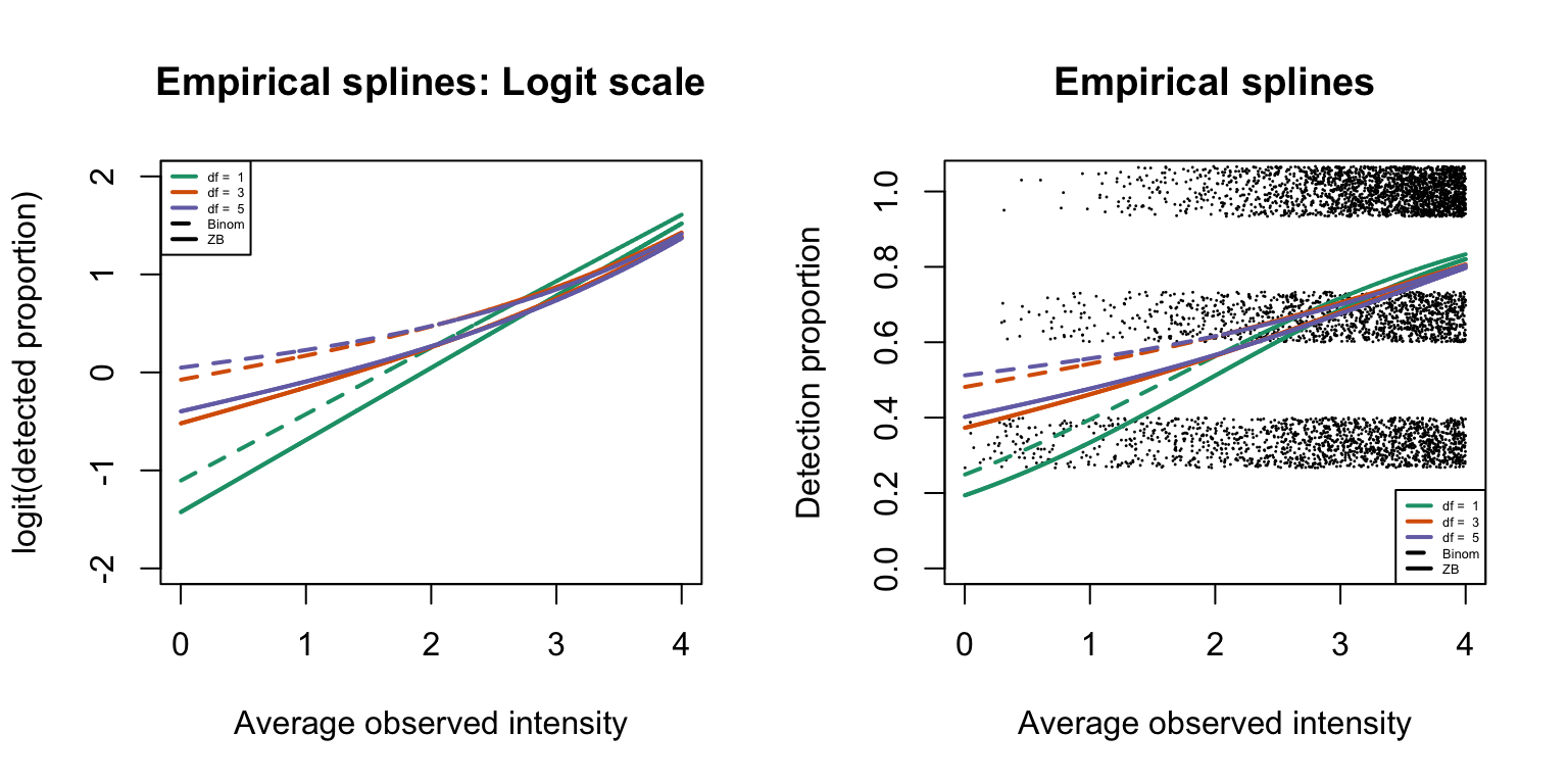

The above plots correspond to Figure S2 of the manuscript.

Reduced deviance compared to an intercept model

The amount of reduced deviance by each logistic spline compared to an intercept model is calculated. The total amount of reduced deviance is calculated as the difference between the largest model with 5 degrees of freedom and the intercept model. As more degrees of freedom is freed up, reduced deviance decreases. The percentage of reduced deviance out of total reduced deviance is calculated for each fitted spline.

params0 <- logitSplines_start(dp = nuis$dp, mu = nuis$mu_obs,
    wt = nuis$wt, df = 0)
baselineFit <- logit_ztbinom(dp = nuis$dp, X = params0$X, wt = nuis$wt,
    beta0 = params0$betas_start)
baselineDev <- 2 * min(baselineFit$info[, "neg.LL"])
devs <- data.frame(df = c(0, dfList), dev = c(baselineDev, sapply(allFits,
    function(i) 2 * min(i$info[, "neg.LL"])))) %>%
    mutate(dev.decre = baselineDev - dev, percDevReduced = dev.decre/max(dev.decre))
ggplot(slice(devs, 2:4), aes(x = df, y = percDevReduced)) + geom_point() +
    geom_line() + geom_text(aes(label = signif(percDevReduced,
    2)), vjust = -0.8) + scale_x_continuous(breaks = c(1, 3,
    5)) + labs(x = "d.f.", y = "Reduced deviance(%)") + ylim(0.95,
    1) + theme_classic()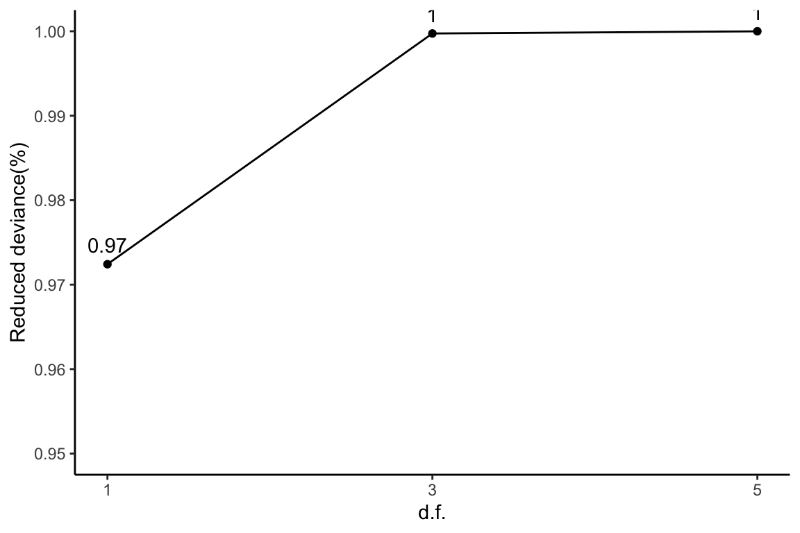

This plot corresponds to Table 1 of the manuscript.

Empirical logit-linear curve with capped probabilities

Next we allow missingness completely at random (MCAR) to present in data. The probability of detection for any observation in a dataset is capped at a value \(\alpha \in (0, 1]\). In other words, we allow a proportion of (1-\(\alpha\)) observations in data to be missing completely at random.

params0 <- logitSplines_start(dp = nuis$dp, mu = nuis$mu_obs,
    wt = nuis$wt, df = 1)
cappedLinear <- cappedLogit_ztbinom(dp = nuis$dp, X = params0$X,
    wt = nuis$wt, alpha0 = 0.9, beta0 = params0$betas_start,
    trace = FALSE)
round(cappedLinear$params, 2)
alpha    b0    b1 
 1.00 -1.56 15.26 
plotEmpSplines(nuis, X = params0$X, cappedLinear$params, capped = TRUE,
    lineCol = lineColours[1], ylim = c(0, 1.04))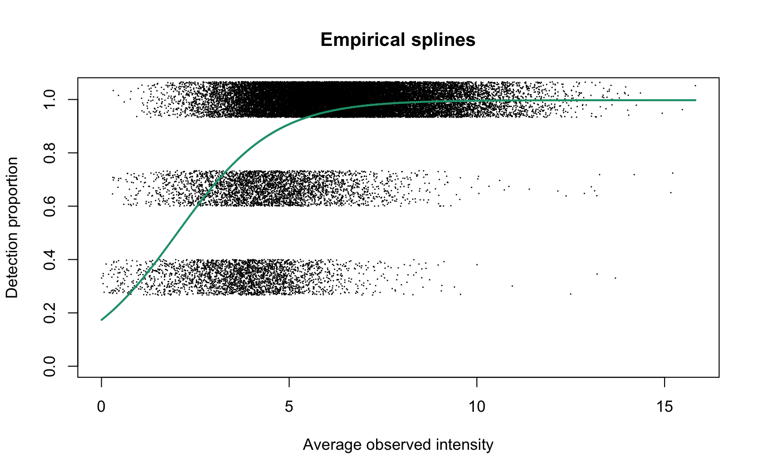

The estimated value of \(\alpha\) is approximately 1. This plot corresponds to Panel (a) in Figure S3 of the manuscript.

Detection probability curve assuming normal observed intensities

dpcFit <- dpc(dat)
plotDPC(dpcFit, ylim = c(0, 1.04))

This plot corresponds to Panel (a) in Figure 2 of the manuscript. The estimated parameters are

round(dpcFit$beta, 2)
   b0    b1 
-1.39  0.73

Dataset B: Cell cycle proteomes

Single cell proteomes were profiled by the true single-cell-derived proteomics (T-SCP) pipeline as described in Brunner et al. (2022). Processed data were downloaded from the ProteomeXchange Consortium via the PRIDE partner repository with the dataset identifier PXD024043. Intensity values of zero were filtered.

Data summary

We first apply a log2-transformation on the precursor-level intensities:

data("datasetB")
dat <- log2(datasetB$prec)
dim(dat)
[1] 10754   231

The overall proportion of missing data is

sum(is.na(dat))/length(dat)
[1] 0.6039

The same analyses as those of Dataset A are also performed on Dataset B on the precursor level. For simplicity, we created a wrapper function to collect all results for a log2-transformed dataset:

diapasefRes <- gatherResults(dat)

Empirical logistic splines for detected proportions

for (i in 1:length(dfList)) {
    if (i == 1)
        plotEmpSplines(diapasefRes$nuis, X = diapasefRes$splineFits_params0[[i]]$X,
            diapasefRes$splineFits[[i]]$params, point.cex = 0.1,
            lineCol = lineColours[i], add.jitter = FALSE)
    if (i > 1)
        plotEmpSplines(diapasefRes$nuis, X = diapasefRes$splineFits_params0[[i]]$X,
            diapasefRes$splineFits[[i]]$params, lineCol = lineColours[i],
            newPlot = FALSE)
}
legend("bottomright", legend = paste("df = ", dfList), col = lineColours,
    lwd = 2, lty = 1, cex = 0.8)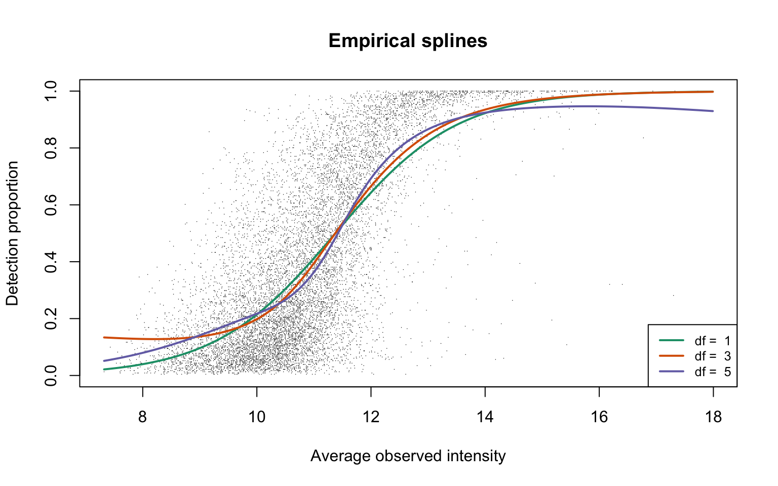

This plot corresponds to Panel (b) in Figure 1 of the manuscript.

Reduced deviance compared to an intercept model

ggplot(slice(diapasefRes$devs, 2:4), aes(x = df, y = percDevReduced)) +
    geom_point() + geom_line() + geom_text(aes(label = signif(percDevReduced,
    2)), vjust = -0.8) + scale_x_continuous(breaks = c(1, 3,
    5)) + labs(x = "d.f.", y = "Reduced deviance(%)") + ylim(0.9,
    1) + theme_classic()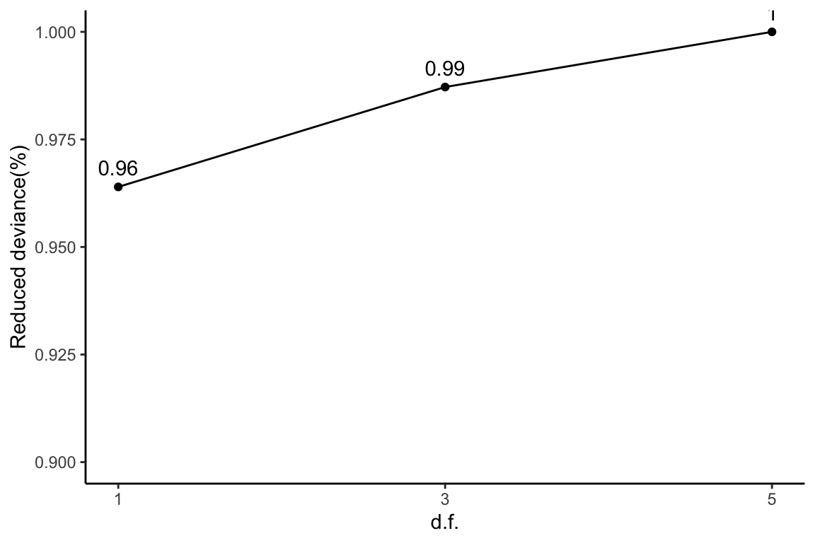

This plot corresponds to Table 1 of the manuscript.

Empirical logit-linear curve with capped probabilities

plotEmpSplines(diapasefRes$nuis, X = diapasefRes$splineFits_params0[[1]]$X,
    diapasefRes$cappedLinearFit$params, capped = TRUE, lineCol = lineColours[1],
    add.jitter = FALSE, point.cex = 0.1)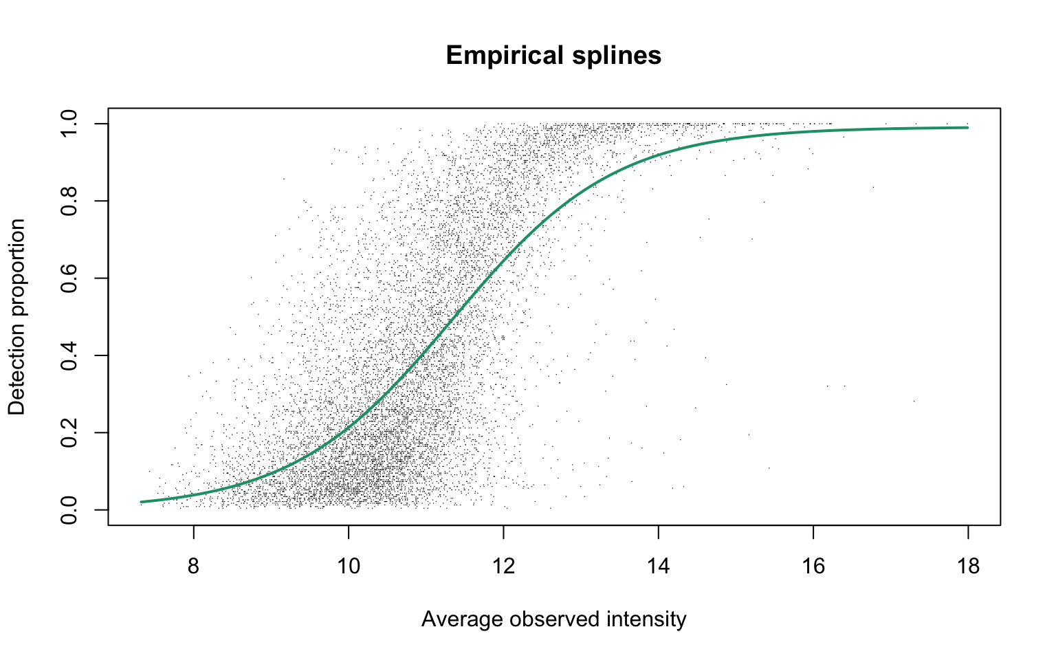

Parameters of the fitted curve are as follows:

round(diapasefRes$cappedLinearFit$params, 2)
alpha    b0    b1 
 0.99 -3.86 12.74

This plot corresponds to Panel (b) in Figure S3 of the manuscript.

Detection probability curve assuming normal observed intensities

plotDPC(diapasefRes$dpcFit, add.jitter = FALSE, point.cex = 0.1)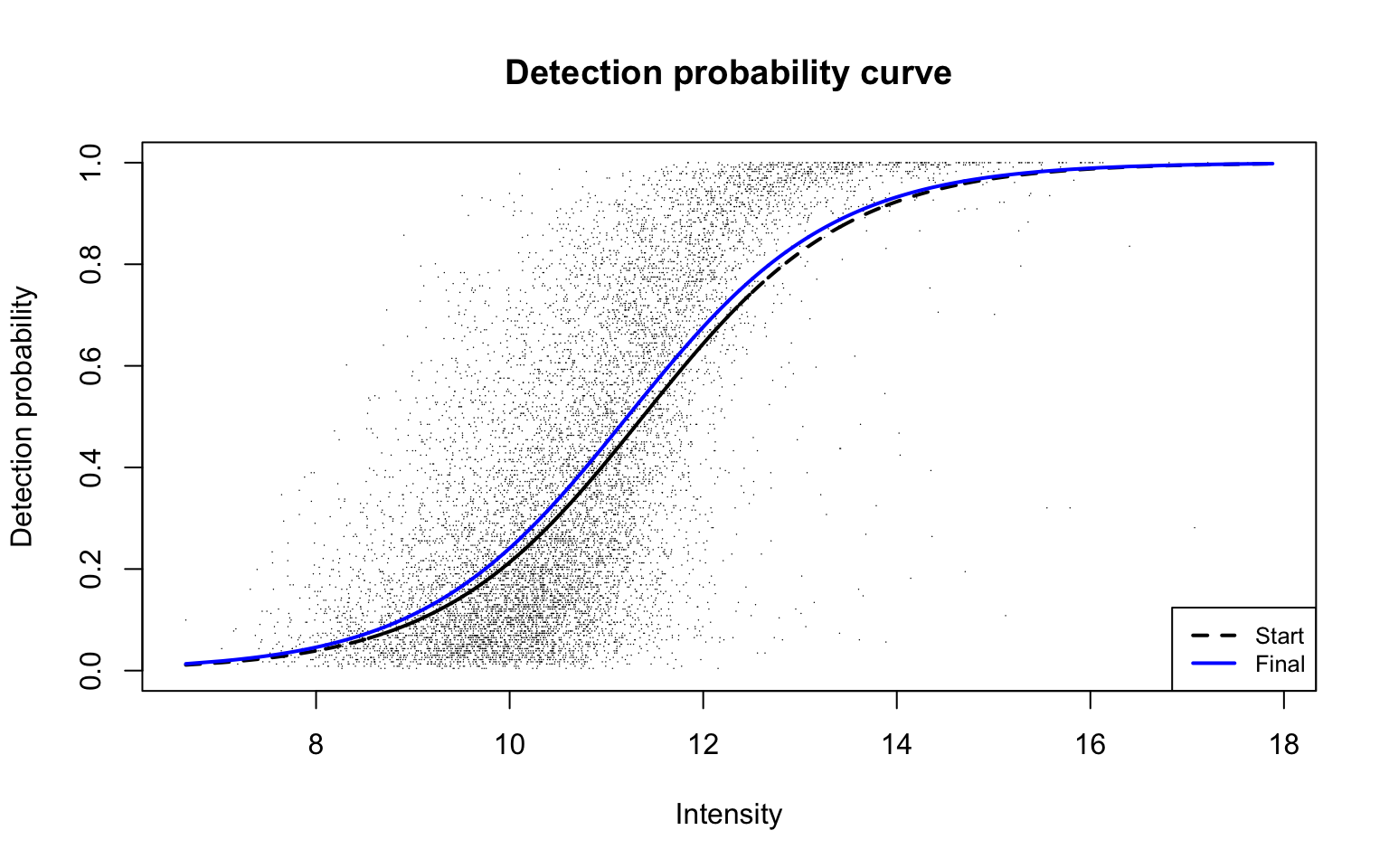

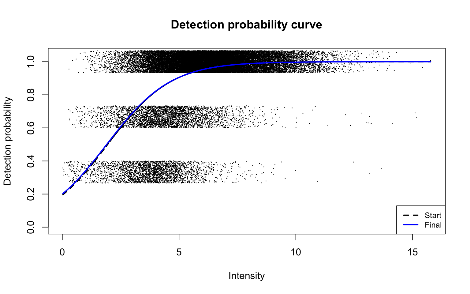
This plot corresponds to Panel (b) in Figure 2 of the manuscript with estimated parameters

round(diapasefRes$dpcFit$beta, 2)
    b0     b1 
-10.57   0.94

Dataset C: HepG2 technical replicate data

Technical replicates of HepG2 cell lysates were analysed in Sinitcyn et al. (2021). MS data were acquired by DIA and analysed by MaxDIA, a DIA data processing software within the MaxQuant environment (Sinitcyn et al. 2021). We downloaded processed data from the ProteomeXchange Consortium via the PRIDE partner repository with the dataset identifier PXD022589.

Data summary

We start the workflow again by applying log2-transformation to the precursor-level intensities.

data("datasetC")
dat <- log2(datasetC$prec)
dim(dat)
[1] 62515    27

The overall proportion of missing data is equal to

sum(is.na(dat))/length(dat)
[1] 0.3284

Empirical logistic splines for detected proportions

maxdiaRes <- gatherResults(dat)
for (i in 1:length(dfList)) {
    if (i == 1)
        plotEmpSplines(maxdiaRes$nuis, X = maxdiaRes$splineFits_params0[[i]]$X,
            maxdiaRes$splineFits[[i]]$params, point.cex = 0.1,
            lineCol = lineColours[i], jitter.amount = 1/ncol(dat)/2)
    if (i > 1)
        plotEmpSplines(maxdiaRes$nuis, X = maxdiaRes$splineFits_params0[[i]]$X,
            maxdiaRes$splineFits[[i]]$params, lineCol = lineColours[i],
            newPlot = FALSE)
}
legend("bottomright", legend = paste("df = ", dfList), col = lineColours,
    lwd = 2, lty = 1, cex = 0.8)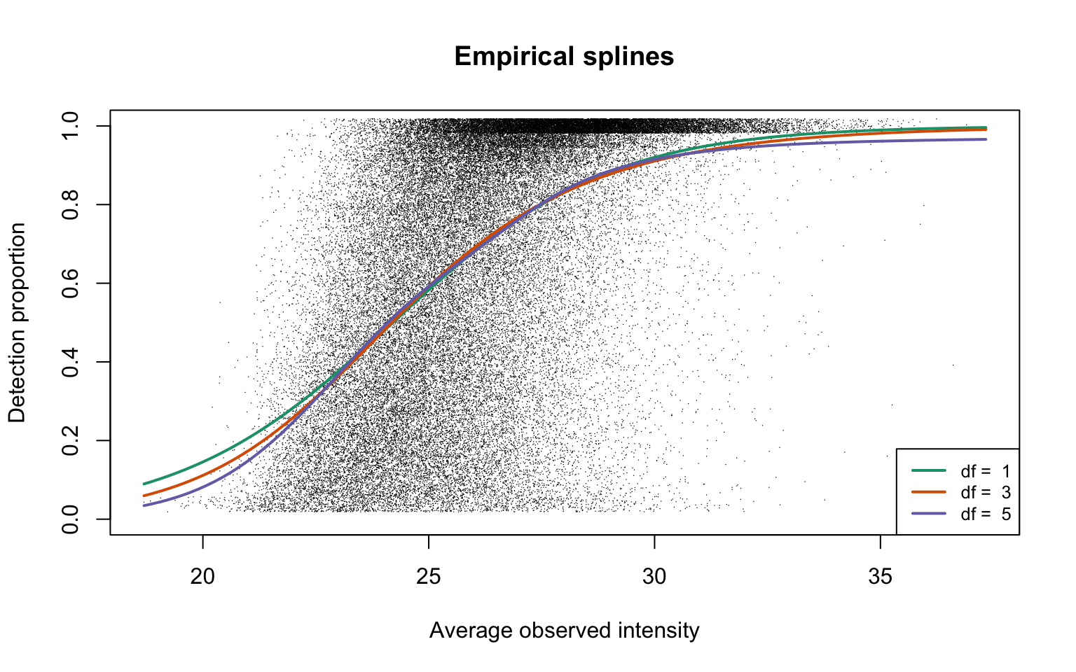

This plot is Panel (c) in Figure 1 in the manuscript.

Reduced deviance compared to an intercept model

ggplot(slice(maxdiaRes$devs, 2:4), aes(x = df, y = percDevReduced)) +
    geom_point() + geom_line() + geom_text(aes(label = signif(percDevReduced,
    2)), vjust = -0.8) + scale_x_continuous(breaks = c(1, 3,
    5)) + labs(x = "d.f.", y = "Reduced deviance(%)") + ylim(0.9,
    1) + theme_classic()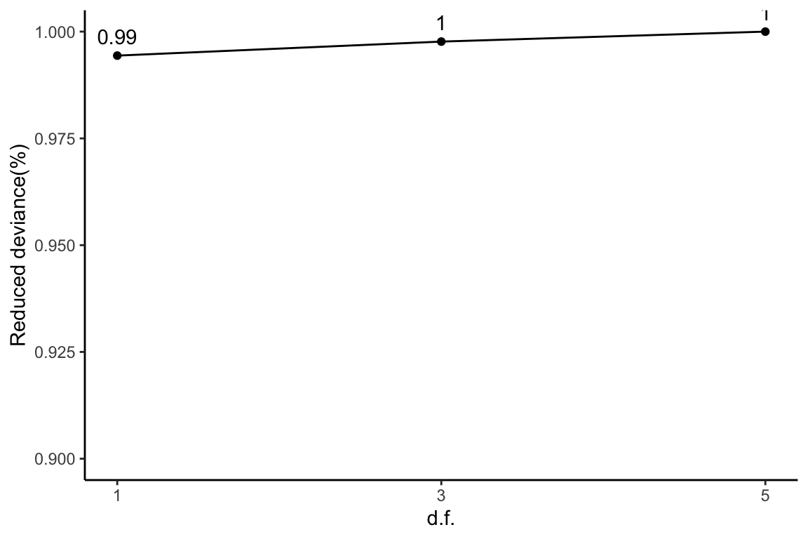

This plot corresponds to Table 1 of the manuscript.

Empirical logit-linear curve with capped probabilities

plotEmpSplines(maxdiaRes$nuis, X = maxdiaRes$splineFits_params0[[1]]$X,
    maxdiaRes$cappedLinearFit$params, capped = TRUE, lineCol = lineColours[1],
    jitter.amount = 1/ncol(dat)/2, point.cex = 0.1)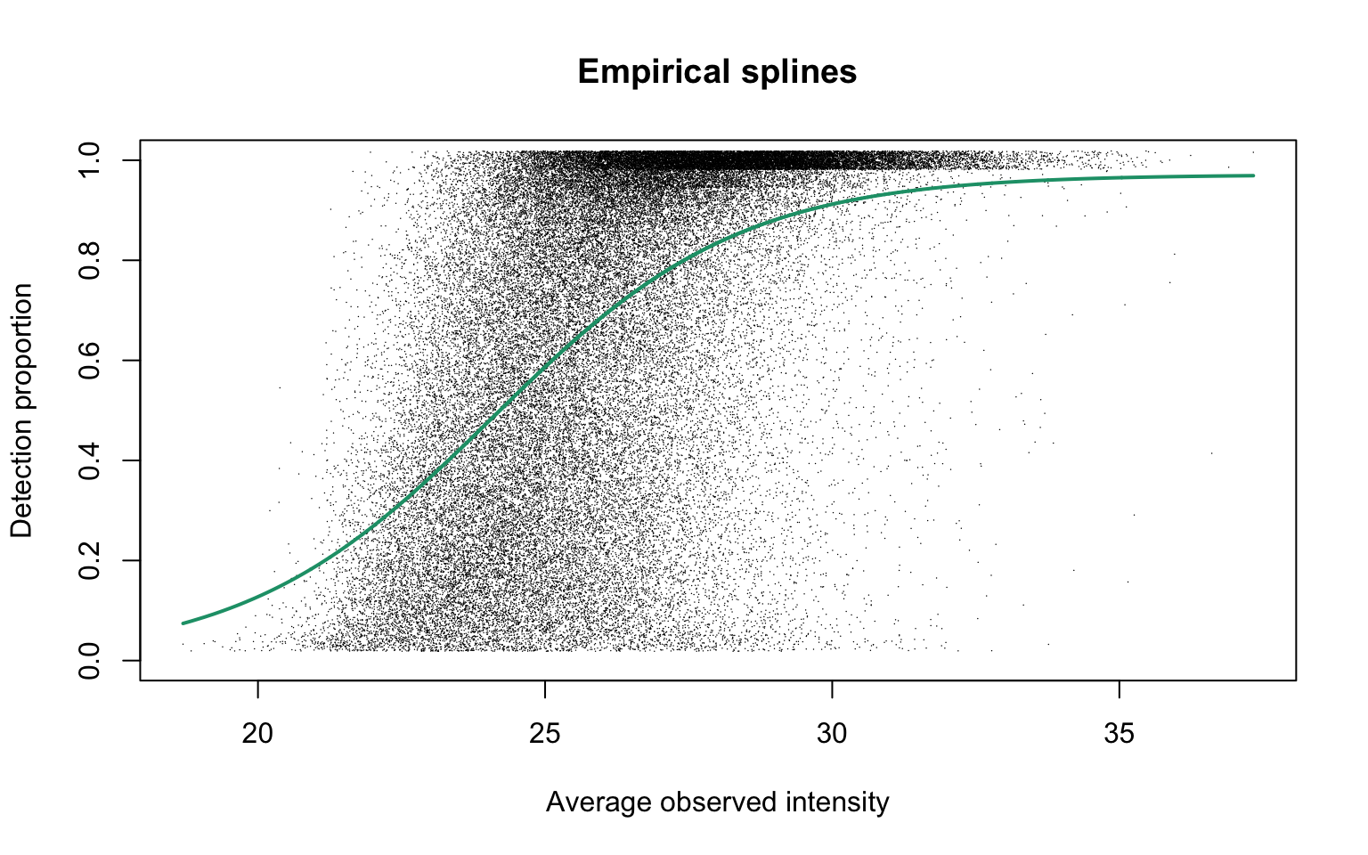

This plot is Panel (c) in Figure S3 in the manuscript with estimated parameters being

round(maxdiaRes$cappedLinearFit$params, 2)
alpha    b0    b1 
 0.97 -2.49 10.75

Detection probability curve assuming normal observed intensities

plotDPC(maxdiaRes$dpcFit, jitter.amount = 1/ncol(dat)/2, point.cex = 0.1)

This plot is Panel (c) in Figure 2 in the manuscript with estimated parameters being

round(maxdiaRes$dpcFit$beta, 2)
    b0     b1 
-10.41   0.43

Dataset D: Human blood plasma proteome

Human blood plasma samples from acute inflammation patients were analysed in Prianichnikov et al. (2020). MS data were acquired by DDA and analysed by MaxQuant. Processed data are available from the ProteomeXchange Consortium via the PRIDE partner repository with the dataset identifier PXD014777.

Data summary

Precursor-level intensity values are first log2-transformed.

data("datasetD")
dat <- log2(datasetD$prec)
dim(dat)
[1] 2384  212

The overall proportion of missing data is equal to

sum(is.na(dat))/length(dat)
[1] 0.5687

Empirical logistic splines for detected proportions

ddaPlasmaRes <- gatherResults(dat)
for (i in 1:length(dfList)) {
    if (i == 1)
        plotEmpSplines(ddaPlasmaRes$nuis, X = ddaPlasmaRes$splineFits_params0[[i]]$X,
            ddaPlasmaRes$splineFits[[i]]$params, lineCol = lineColours[i],
            add.jitter = FALSE)
    if (i > 1)
        plotEmpSplines(ddaPlasmaRes$nuis, X = ddaPlasmaRes$splineFits_params0[[i]]$X,
            ddaPlasmaRes$splineFits[[i]]$params, lineCol = lineColours[i],
            newPlot = FALSE)
}
legend("bottomright", legend = paste("df = ", dfList), col = lineColours,
    lwd = 2, lty = 1)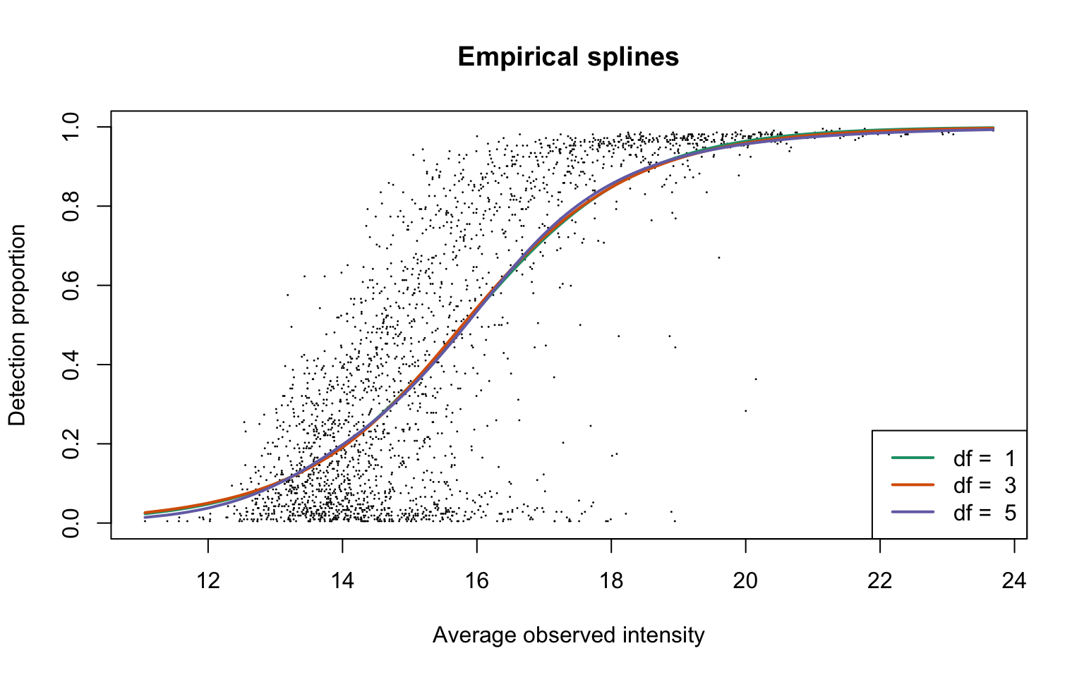

This plot is Panel (d) in Figure 1 in the main text.

Reduced deviance compared to an intercept model

ggplot(slice(ddaPlasmaRes$devs, 2:4), aes(x = df, y = percDevReduced)) +
    geom_point() + geom_line() + geom_text(aes(label = signif(percDevReduced,
    2)), vjust = -0.8) + scale_x_continuous(breaks = c(1, 3,
    5)) + labs(x = "d.f.", y = "Reduced deviance(%)") + ylim(0.9,
    1) + theme_classic()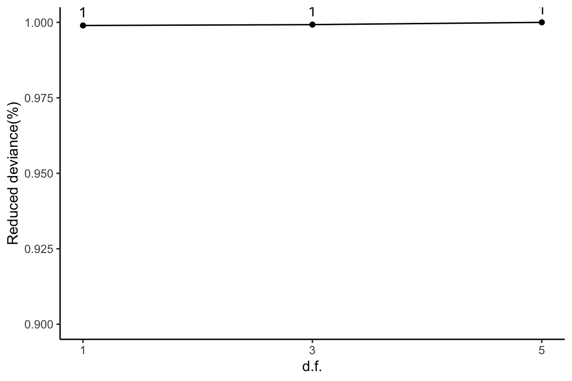

This plot corresponds to Table 1 from the main text.

Empirical logit-linear curve with capped probabilities

plotEmpSplines(ddaPlasmaRes$nuis, X = ddaPlasmaRes$splineFits_params0[[1]]$X,
    ddaPlasmaRes$cappedLinearFit$params, capped = TRUE, lineCol = lineColours[1],
    add.jitter = FALSE)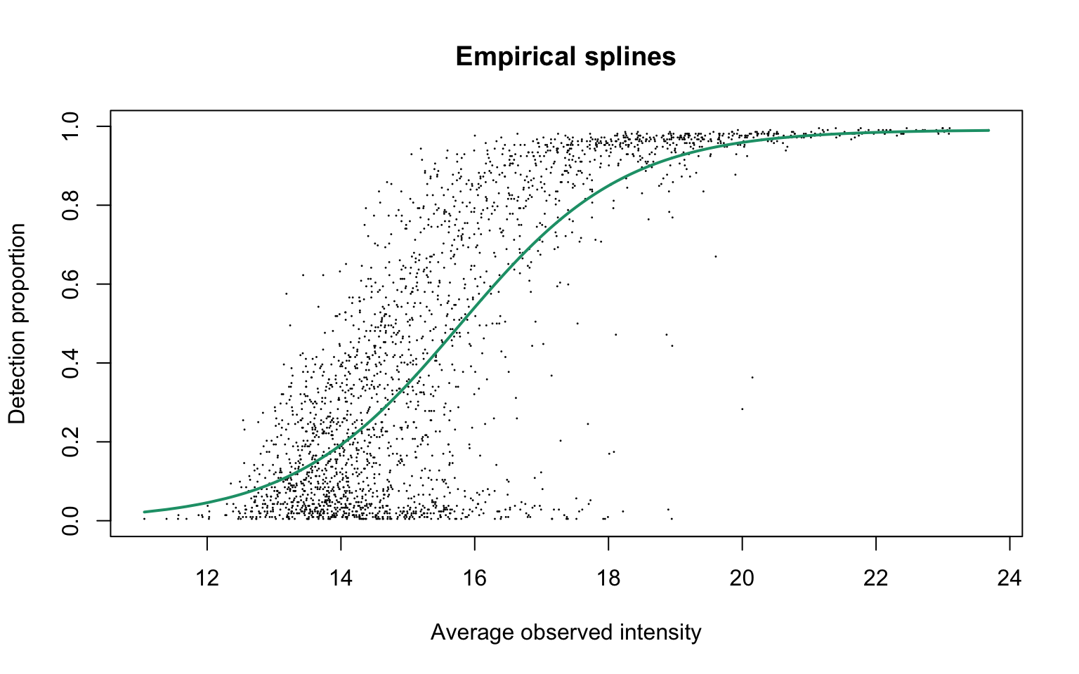

This plot is Panel (d) in Figure S3 of the manuscript, with estimated parameters being

round(ddaPlasmaRes$cappedLinearFit$params, 2)
alpha    b0    b1 
 0.99 -3.78 12.64

Detection probability curve assuming normal observed intensities

plotDPC(ddaPlasmaRes$dpcFit, add.jitter = FALSE)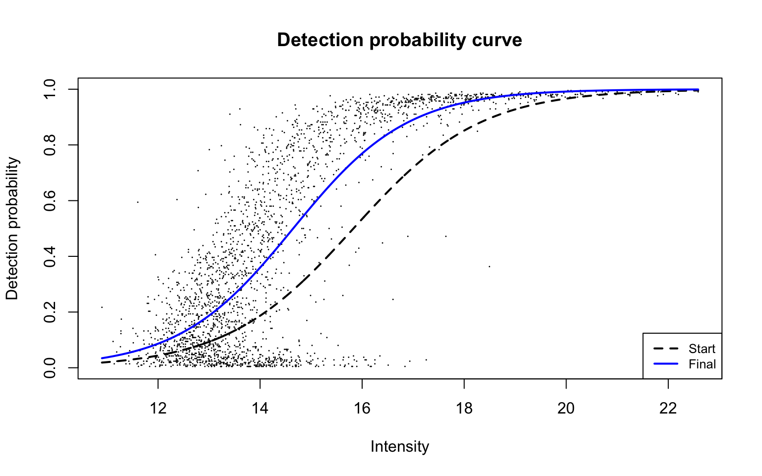

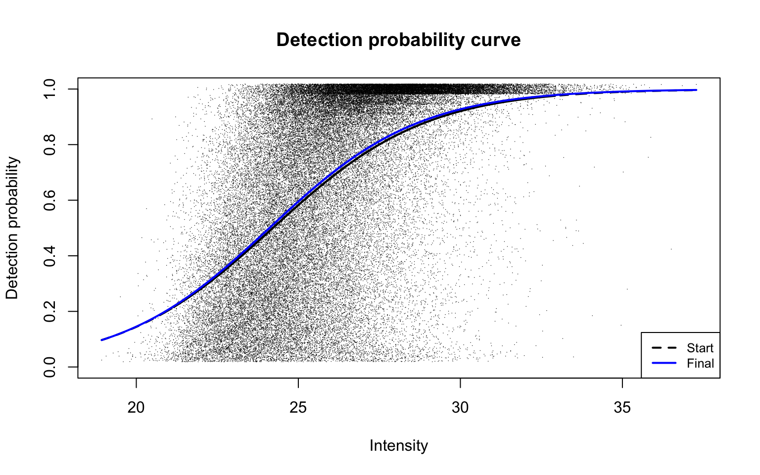
This plot is Panel (d) in Figure 2 of the manuscript, with estimated parameters being

round(ddaPlasmaRes$dpcFit$beta, 2)
    b0     b1 
-13.05   0.89

References

Brunner, Andreas-David, Marvin Thielert, Catherine Vasilopoulou, Constantin Ammar, Fabian Coscia, Andreas Mund, Ole B Hoerning, et al. 2022. “Ultra-High Sensitivity Mass Spectrometry Quantifies Single-Cell Proteome Changes Upon Perturbation.” Molecular Systems Biology 18 (3): e10798.

Demichev, Vadim, Christoph B Messner, Spyros I Vernardis, Kathryn S Lilley, and Markus Ralser. 2020. “DIA-NN: Neural Networks and Interference Correction Enable Deep Proteome Coverage in High Throughput.” Nature Methods 17 (1): 41–44.

Navarro, Pedro, Jörg Kuharev, Ludovic C Gillet, Oliver M Bernhardt, Brendan MacLean, Hannes L Röst, Stephen A Tate, et al. 2016. “A Multicenter Study Benchmarks Software Tools for Label-Free Proteome Quantification.” Nature Biotechnology 34 (11): 1130–36.

Prianichnikov, Nikita, Heiner Koch, Scarlet Koch, Markus Lubeck, Raphael Heilig, Sven Brehmer, Roman Fischer, and Jürgen Cox. 2020. “MaxQuant Software for Ion Mobility Enhanced Shotgun Proteomics.” Molecular & Cellular Proteomics 19 (6): 1058–69.

Sinitcyn, Pavel, Hamid Hamzeiy, Favio Salinas Soto, Daniel Itzhak, Frank McCarthy, Christoph Wichmann, Martin Steger, et al. 2021. “MaxDIA Enables Library-Based and Library-Free Data-Independent Acquisition Proteomics.” Nature Biotechnology 39 (12): 1563–73.

Session information

sessionInfo()
R version 4.3.1 (2023-06-16)
Platform: x86_64-apple-darwin20 (64-bit)
Running under: macOS Ventura 13.5.2

Matrix products: default
BLAS:   /Library/Frameworks/R.framework/Versions/4.3-x86_64/Resources/lib/libRblas.0.dylib 
LAPACK: /Library/Frameworks/R.framework/Versions/4.3-x86_64/Resources/lib/libRlapack.dylib;  LAPACK version 3.11.0

locale:
[1] en_US.UTF-8/en_US.UTF-8/en_US.UTF-8/C/en_US.UTF-8/en_US.UTF-8

time zone: Australia/Melbourne
tzcode source: internal

attached base packages:
[1] stats     graphics  grDevices utils     datasets  methods   base     

other attached packages:
 [1] protDP_1.1.0    lubridate_1.9.3 forcats_1.0.0   stringr_1.5.0   dplyr_1.1.3     purrr_1.0.2    
 [7] readr_2.1.4     tidyr_1.3.0     tibble_3.2.1    ggplot2_3.4.3   tidyverse_2.0.0

loaded via a namespace (and not attached):
 [1] sass_0.4.7         utf8_1.2.3         generics_0.1.3     stringi_1.7.12     hms_1.1.3         
 [6] digest_0.6.33      magrittr_2.0.3     RColorBrewer_1.1-3 timechange_0.2.0   evaluate_0.22     
[11] grid_4.3.1         fastmap_1.1.1      rprojroot_2.0.3    jsonlite_1.8.7     limma_3.57.9      
[16] formatR_1.14       fansi_1.0.5        scales_1.2.1       textshaping_0.3.7  jquerylib_0.1.4   
[21] cli_3.6.1          rlang_1.1.1        splines_4.3.1      munsell_0.5.0      withr_2.5.1       
[26] cachem_1.0.8       yaml_2.3.7         tools_4.3.1        tzdb_0.4.0         memoise_2.0.1     
[31] colorspace_2.1-0   vctrs_0.6.3        R6_2.5.1           lifecycle_1.0.3    fs_1.6.3          
[36] ragg_1.2.6         pkgconfig_2.0.3    desc_1.4.2         pkgdown_2.0.7      pillar_1.9.0      
[41] bslib_0.5.1        gtable_0.3.4       glue_1.6.2         statmod_1.5.0      systemfonts_1.0.5 
[46] xfun_0.40          tidyselect_1.2.0   rstudioapi_0.15.0  knitr_1.44         farver_2.1.1      
[51] htmltools_0.5.6.1  labeling_0.4.3     rmarkdown_2.25     compiler_4.3.1

Mengbo Li

Overview

Load packages

Dataset A: Hybrid proteome data

Data overview

Empirical logistic splines for detected proportions

Empirical logistic splines assuming the binomial distribution

Reduced deviance compared to an intercept model

Empirical logit-linear curve with capped probabilities

Detection probability curve assuming normal observed intensities

Dataset B: Cell cycle proteomes

Data summary

Empirical logistic splines for detected proportions

Reduced deviance compared to an intercept model

Empirical logit-linear curve with capped probabilities

Detection probability curve assuming normal observed intensities

Dataset C: HepG2 technical replicate data

Data summary

Empirical logistic splines for detected proportions

Reduced deviance compared to an intercept model

Empirical logit-linear curve with capped probabilities

Detection probability curve assuming normal observed intensities

Dataset D: Human blood plasma proteome

Data summary

Empirical logistic splines for detected proportions

Reduced deviance compared to an intercept model

Empirical logit-linear curve with capped probabilities

Detection probability curve assuming normal observed intensities

References

Session information