Supplementary results and figures

Overview

On this page, the analysis workflow presented in the main text is applied on each of the four example datasets on the protein group level. Additionally, two more datasets were downloaded. The same analyses are also performed on both precursor- and protein-levels on these additional datasets.

Load packages

library(tidyverse)
library(protDP)
dfList <- seq(1, 5, 2)
lineColours <- RColorBrewer::brewer.pal(3, "Dark2")

Dataset A: Hybrid proteome data

LFQ intensities summarised by MaxLFQ (Cox et al. 2014) were extracted from the DIA-NN (Demichev et al. 2020) output on the protein group level. The log2-transformation is applied to LFQ intensities.

Data overview

data("datasetA")
dat <- log2(datasetA$prot)
dim(dat)
[1] 5974    3

The overall proportion of missing data on the protein level is equal to

sum(is.na(dat))/length(dat)
[1] 0.0505

Empirical logistic splines for detected proportions

hyeProt <- gatherResults(dat)
for (i in 1:length(dfList)) {
    if (i == 1)
        plotEmpSplines(hyeProt$nuis, X = hyeProt$splineFits_params0[[i]]$X,
            hyeProt$splineFits[[i]]$params, lineCol = lineColours[i],
            point.cex = 0.15, ylim = c(0, 1.04))
    if (i > 1)
        plotEmpSplines(hyeProt$nuis, X = hyeProt$splineFits_params0[[i]]$X,
            hyeProt$splineFits[[i]]$params, lineCol = lineColours[i],
            newPlot = FALSE)
}
legend("bottomright", legend = paste("df = ", dfList), col = lineColours,
    lwd = 2, lty = 1, cex = 0.8)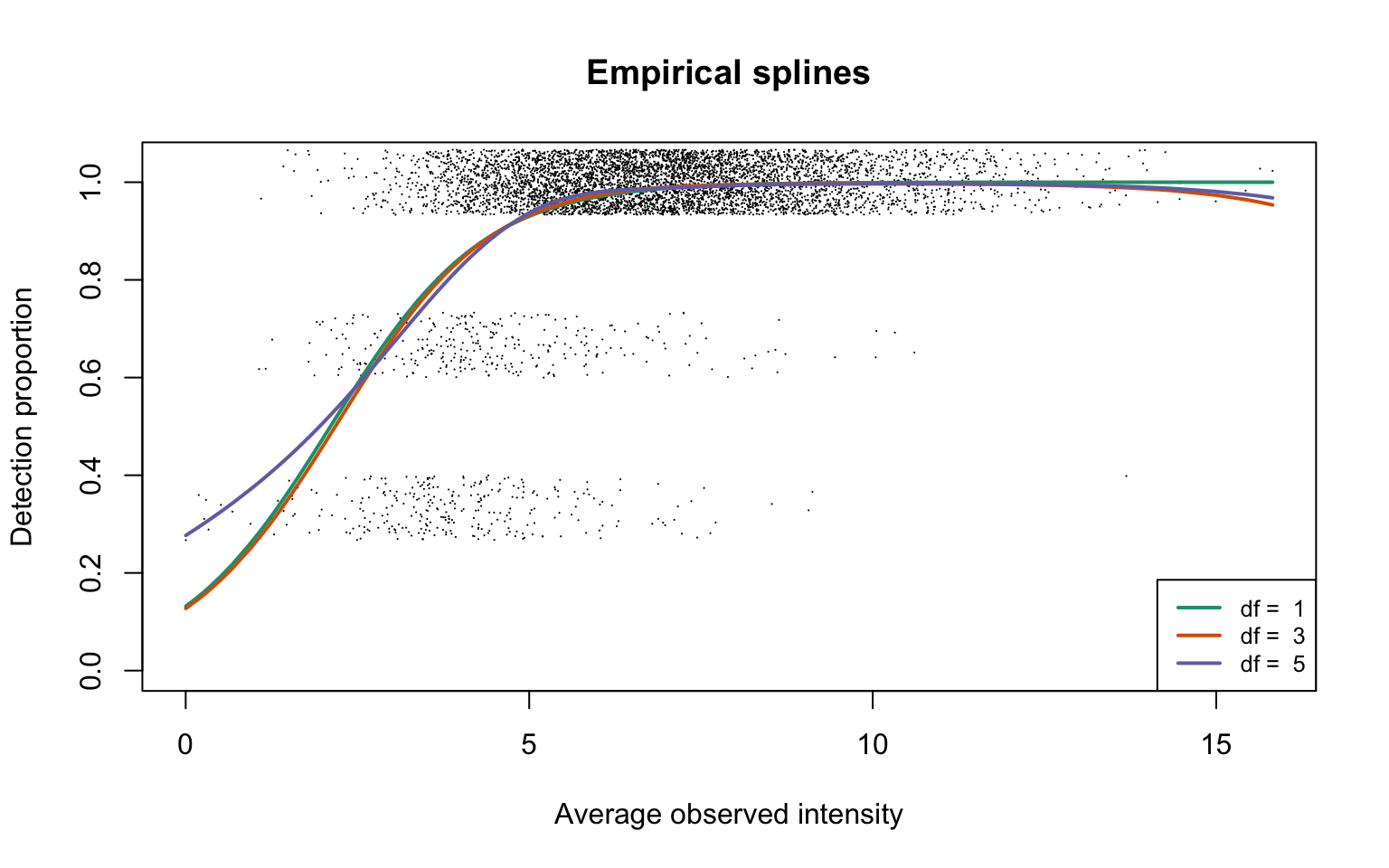

Reduced deviance compared to an intercept model

ggplot(slice(hyeProt$devs, 2:4), aes(x = df, y = percDevReduced)) +
    geom_point() + geom_line() + geom_text(aes(label = signif(percDevReduced,
    2)), vjust = -0.8) + scale_x_continuous(breaks = c(1, 3,
    5)) + labs(x = "d.f.", y = "Reduced deviance(%)") + ylim(0.9,
    1) + theme_classic()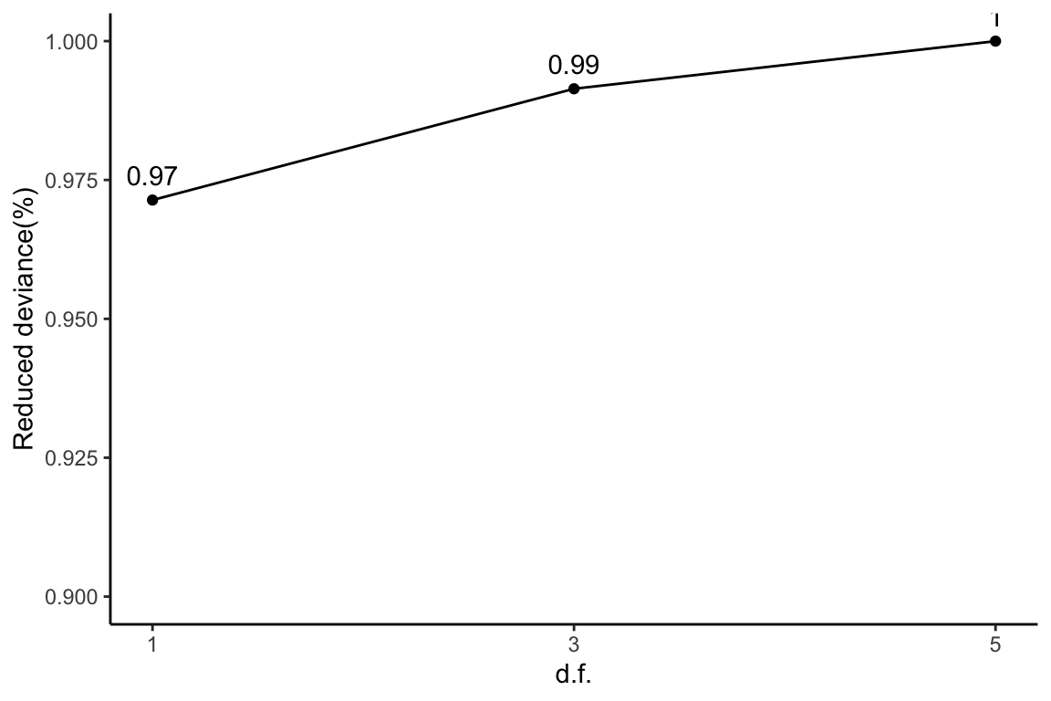

Empirical logit-linear curve with capped probabilities

plotEmpSplines(hyeProt$nuis, X = hyeProt$splineFits_params0[[1]]$X,
    hyeProt$cappedLinearFit$params, capped = TRUE, lineCol = lineColours[1],
    ylim = c(0, 1.04), point.cex = 0.15)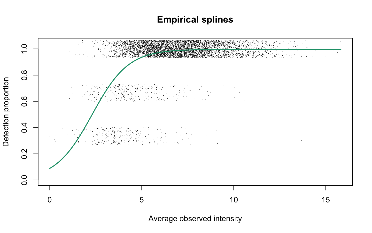

The estimated parameters are

round(hyeProt$cappedLinearFit$params, 2)
alpha    b0    b1 
 1.00 -2.33 19.98

We see that the estimated \(\alpha\) value is 1.

Detection probability curve assuming normal observed intensities

plotDPC(hyeProt$dpcFit, jitter.amount = NULL, point.cex = 0.15,
    ylim = c(0, 1.04))

The estimated parameters for the detection probability curve are

round(hyeProt$dpcFit$beta, 2)
   b0    b1 
-1.79  0.88

Dataset B: Cell cycle proteomes

LFQ intensities summarised by MaxLFQ (Cox et al. 2014) were extracted from the DIA-NN (Demichev et al. 2020) report for protein groups. The log2-transformation is first applied to LFQ intensities.

Data overview

data("datasetB")
dat <- log2(datasetB$prot)
dim(dat)
[1] 2661  231

The overall proportion of missing data on the protein-level is

sum(is.na(dat))/length(dat)
[1] 0.4737

Empirical logistic splines for detected proportions

scProt <- gatherResults(dat, b1.upper = Inf)
for (i in 1:length(dfList)) {
    if (i == 1)
        plotEmpSplines(scProt$nuis, X = scProt$splineFits_params0[[i]]$X,
            scProt$splineFits[[i]]$params, lineCol = lineColours[i],
            add.jitter = FALSE, point.cex = 0.15)
    if (i > 1)
        plotEmpSplines(scProt$nuis, X = scProt$splineFits_params0[[i]]$X,
            scProt$splineFits[[i]]$params, lineCol = lineColours[i],
            newPlot = FALSE)
}
legend("bottomright", legend = paste("df = ", dfList), col = lineColours,
    lwd = 2, lty = 1, cex = 0.8)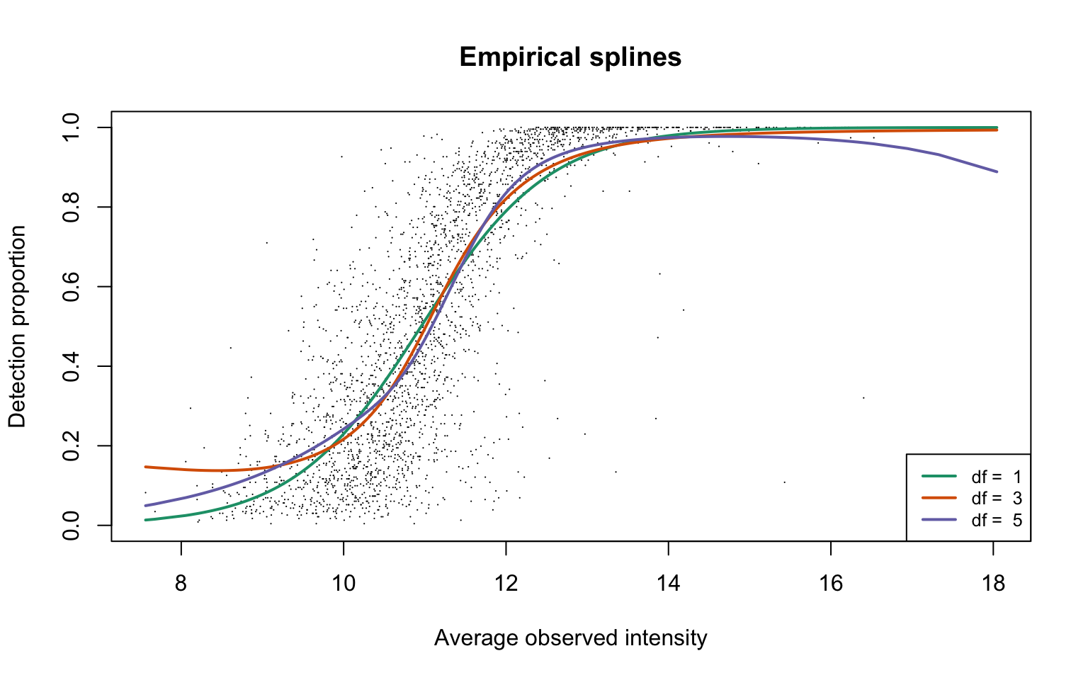

Reduced deviance compared to an intercept model

ggplot(slice(scProt$devs, 2:4), aes(x = df, y = percDevReduced)) +
    geom_point() + geom_line() + geom_text(aes(label = signif(percDevReduced,
    2)), vjust = -0.8) + scale_x_continuous(breaks = c(1, 3,
    5)) + labs(x = "d.f.", y = "Reduced deviance(%)") + ylim(0.9,
    1) + theme_classic()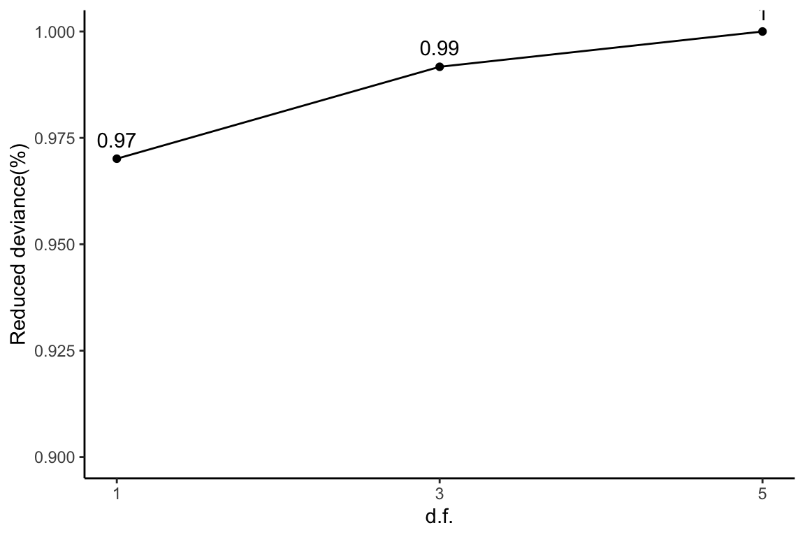

Empirical logit-linear curve with capped probabilities

plotEmpSplines(scProt$nuis, X = scProt$splineFits_params0[[1]]$X,
    scProt$cappedLinearFit$params, capped = TRUE, lineCol = lineColours[1],
    point.cex = 0.15)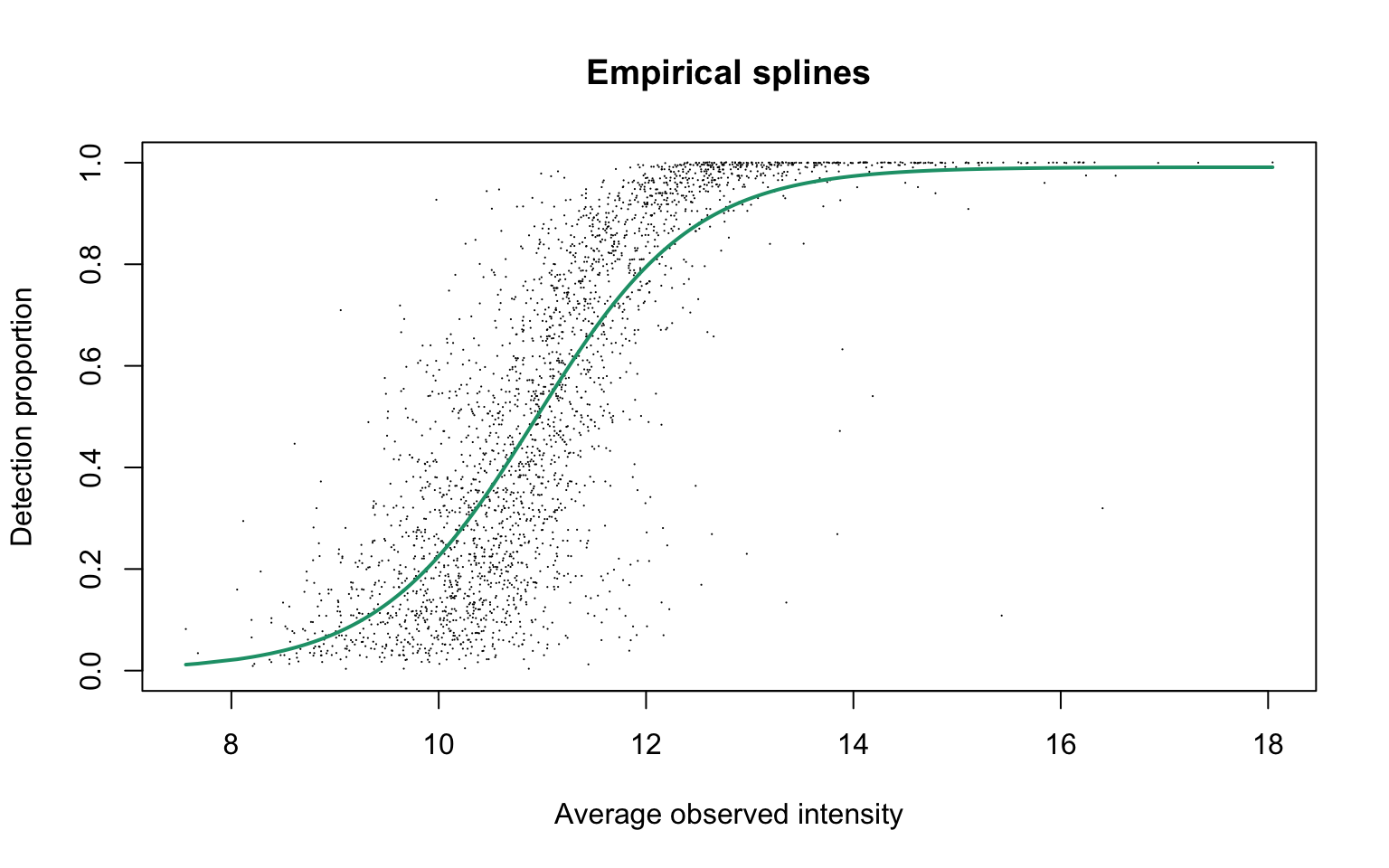

Estimated parameters are

round(scProt$cappedLinearFit$params, 2)
alpha    b0    b1 
 0.99 -4.42 17.13

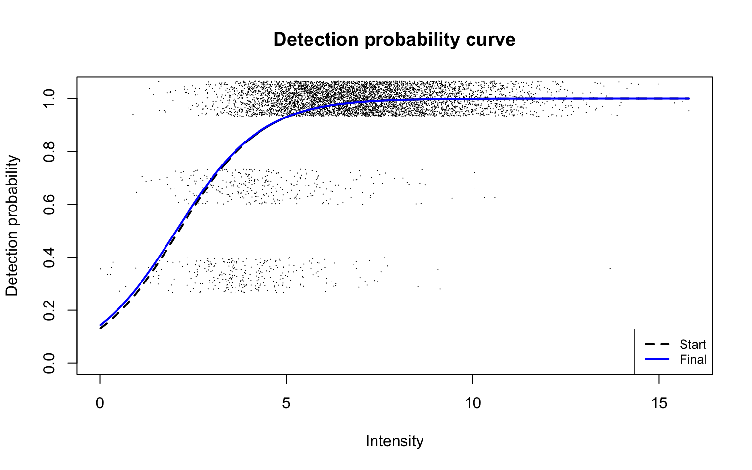
Detection probability curve assuming normal observed intensities

plotDPC(scProt$dpcFit, add.jitter = FALSE, point.cex = 0.1)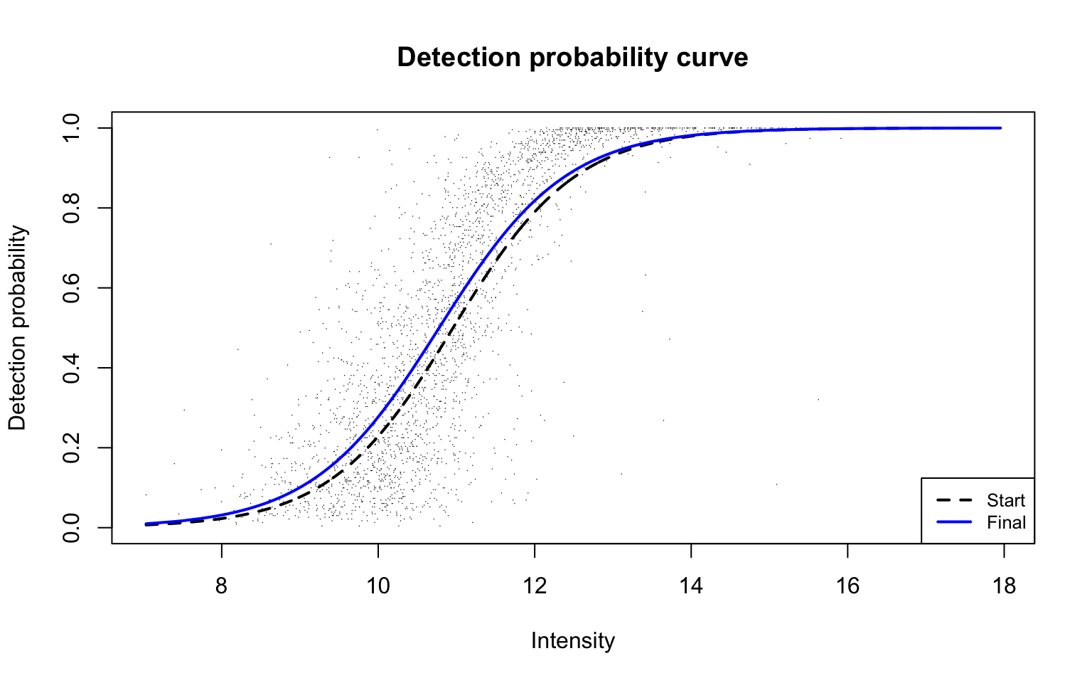

Parameters of the detection probability curve are as follows:

round(scProt$dpcFit$beta, 2)
    b0     b1 
-13.27   1.23

Dataset C: HepG2 technical replicate data

For the protein group level analysis, we use the proteinGroups.txt file from the MaxQuant output. The LFQ intensities are first log2-transformed.

Data overview

data("datasetC")
dat <- log2(datasetC$prot)
dim(dat)
[1] 6282   27

The overall proportion of missingness in protein group level data is

sum(is.na(dat))/length(dat)
[1] 0.05533

Empirical logistic splines for detected proportions

hepg2Prot <- gatherResults(dat)
for (i in 1:length(dfList)) {
    if (i == 1)
        plotEmpSplines(hepg2Prot$nuis, X = hepg2Prot$splineFits_params0[[i]]$X,
            hepg2Prot$splineFits[[i]]$params, lineCol = lineColours[i],
            jitter.amount = 1/ncol(dat)/2)
    if (i > 1)
        plotEmpSplines(hepg2Prot$nuis, X = hepg2Prot$splineFits_params0[[i]]$X,
            hepg2Prot$splineFits[[i]]$params, lineCol = lineColours[i],
            newPlot = FALSE)
}
legend("bottomright", legend = paste("df = ", dfList), col = lineColours,
    lwd = 2, lty = 1, cex = 0.8)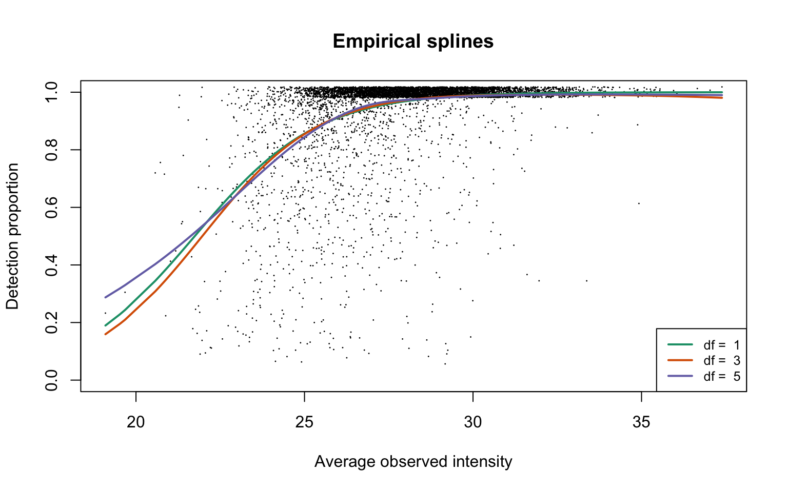

Reduced deviance compared to an intercept model

ggplot(slice(hepg2Prot$devs, 2:4), aes(x = df, y = percDevReduced)) +
    geom_point() + geom_line() + geom_text(aes(label = signif(percDevReduced,
    2)), vjust = -0.8) + scale_x_continuous(breaks = c(1, 3,
    5)) + labs(x = "d.f.", y = "Reduced deviance(%)") + ylim(0.9,
    1) + theme_classic()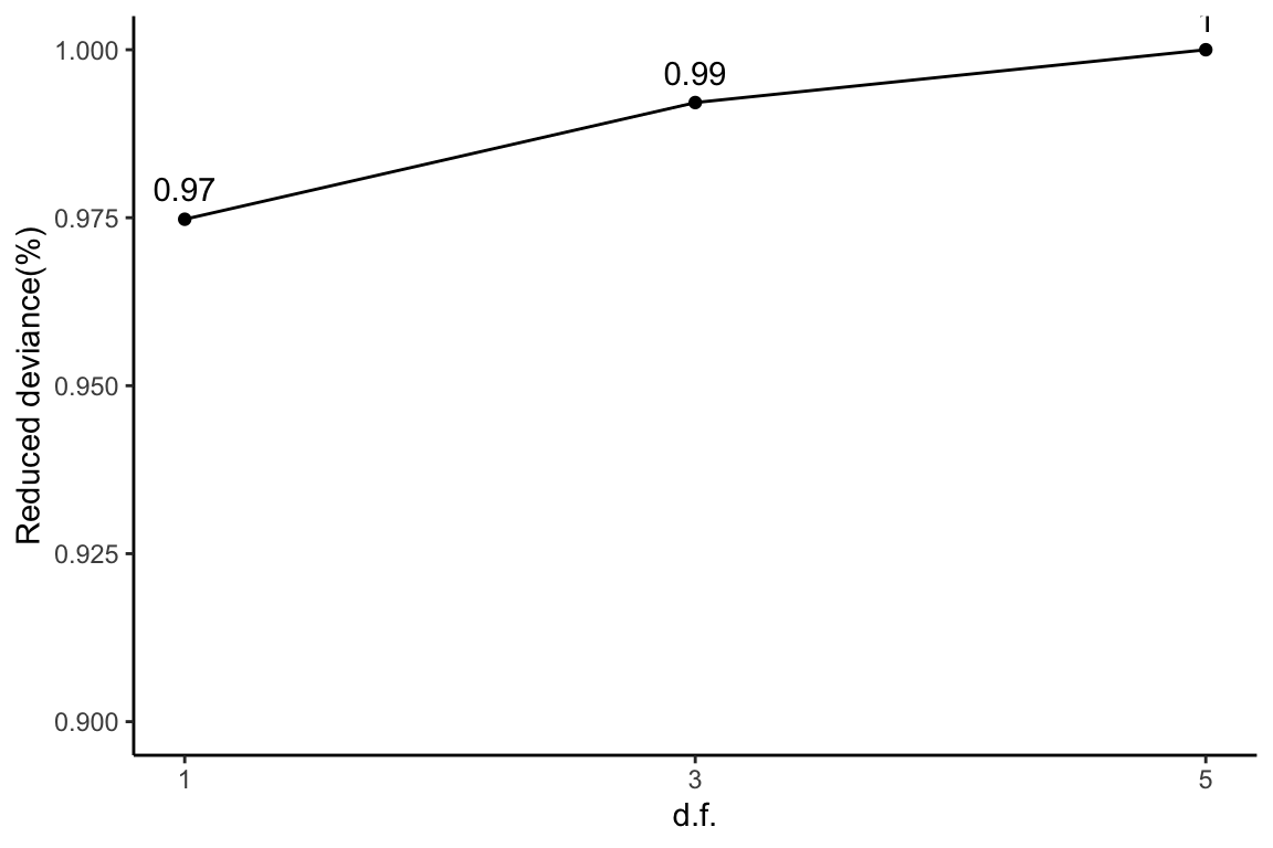

Empirical logit-linear curve with capped probabilities

plotEmpSplines(hepg2Prot$nuis, X = hepg2Prot$splineFits_params0[[1]]$X,
    hepg2Prot$cappedLinearFit$params, capped = TRUE, lineCol = lineColours[1],
    jitter.amount = 1/ncol(dat)/2)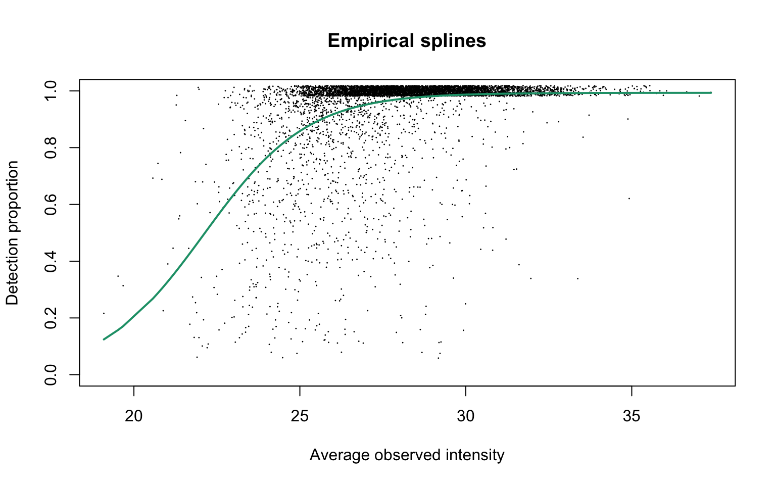

The estimated parameters are

round(hepg2Prot$cappedLinearFit$params, 2)
alpha    b0    b1 
 0.99 -1.94 14.66

Detection probability curve assuming normal observed intensities

plotDPC(hepg2Prot$dpcFit, jitter.amount = 1/ncol(dat)/2)

Parameters of the detection probability curve are

round(hepg2Prot$dpcFit$beta, 2)
    b0     b1 
-11.90   0.55

Dataset D: Human blood plasma proteome

For the protein group level analysis, we use the proteinGroups.txt file from the MaxQuant output downloaded from the ProteomeXchange Consortium via the PRIDE partner repository with the dataset identifier PXD014777.

Data overview

data("datasetD")
dat <- log2(datasetD$prot)
dim(dat)
[1] 332 212

The overall proportion of missing data in the protein group level data is

sum(is.na(dat))/length(dat)
[1] 0.4123

Empirical logistic splines for detected proportions

ddaPlasmaProt <- gatherResults(dat)
for (i in 1:length(dfList)) {
    if (i == 1)
        plotEmpSplines(ddaPlasmaProt$nuis, X = ddaPlasmaProt$splineFits_params0[[i]]$X,
            ddaPlasmaProt$splineFits[[i]]$params, lineCol = lineColours[i],
            add.jitter = FALSE)
    if (i > 1)
        plotEmpSplines(ddaPlasmaProt$nuis, X = ddaPlasmaProt$splineFits_params0[[i]]$X,
            ddaPlasmaProt$splineFits[[i]]$params, lineCol = lineColours[i],
            newPlot = FALSE)
}
legend("bottomright", legend = paste("df = ", dfList), col = lineColours,
    lwd = 2, lty = 1, cex = 0.8)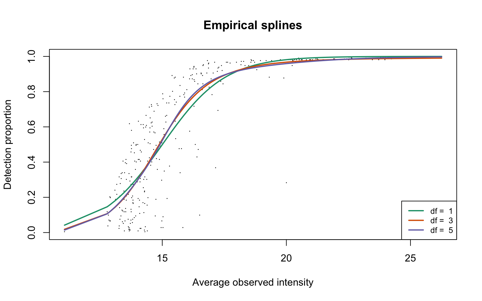

Reduced deviance compared to an intercept model

ggplot(slice(ddaPlasmaProt$devs, 2:4), aes(x = df, y = percDevReduced)) +
    geom_point() + geom_line() + geom_text(aes(label = signif(percDevReduced,
    2)), vjust = -0.8) + scale_x_continuous(breaks = c(1, 3,
    5)) + labs(x = "d.f.", y = "Reduced deviance(%)") + ylim(0.9,
    1) + theme_classic()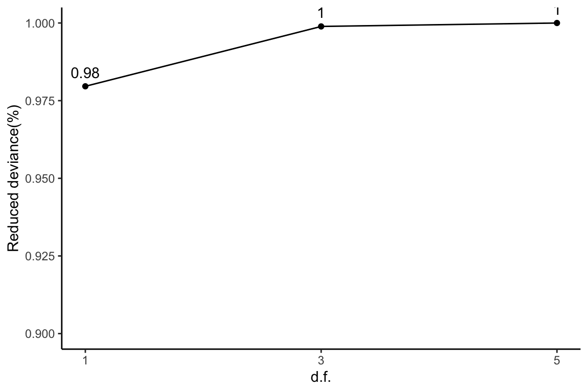

Empirical logit-linear curve with capped probabilities

plotEmpSplines(ddaPlasmaProt$nuis, X = ddaPlasmaProt$splineFits_params0[[1]]$X,
    ddaPlasmaProt$cappedLinearFit$params, capped = TRUE, lineCol = lineColours[1],
    add.jitter = FALSE)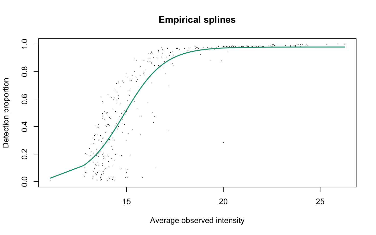

Estimated parameters are

round(ddaPlasmaProt$cappedLinearFit$params, 2)
alpha    b0    b1 
 0.98 -3.65 18.16

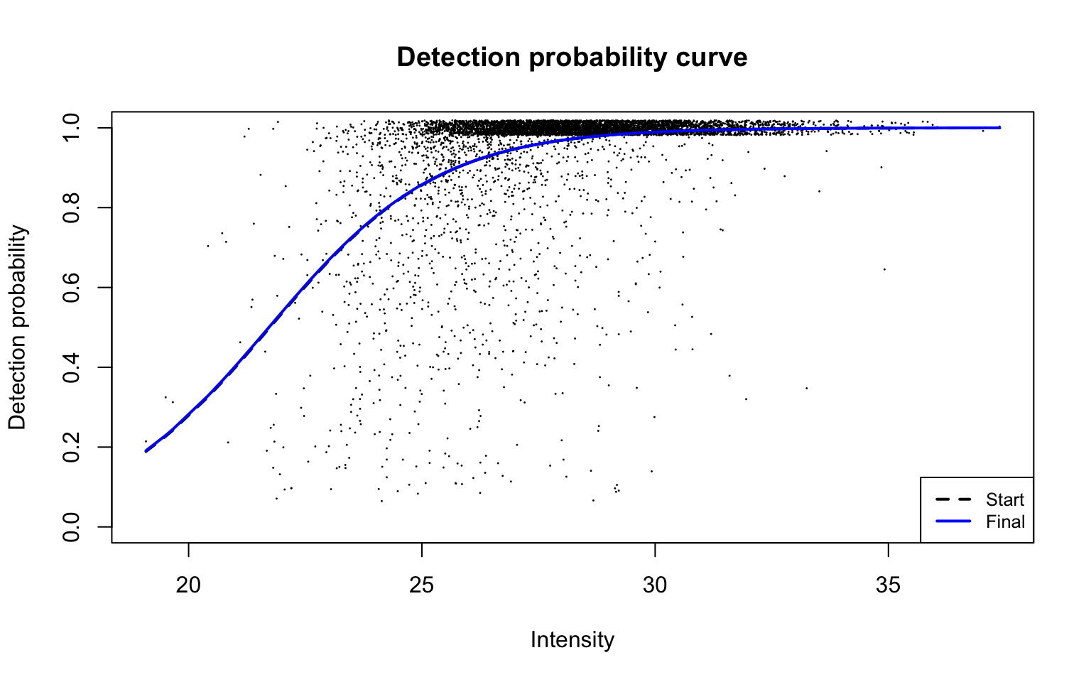
Detection probability curve assuming normal observed intensities

plotDPC(ddaPlasmaProt$dpcFit, add.jitter = FALSE)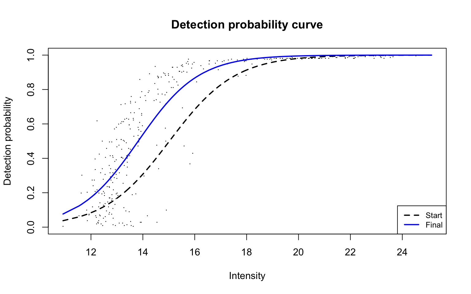

Parameters for the fitted detection probability curve are

round(ddaPlasmaProt$dpcFit$beta, 2)
    b0     b1 
-11.88   0.86

Supplementary dataset: Sydney heart bank data

Cryopreserved left ventricular myocardium samples from the human hearts were analysed. MS data were acquired in DIA mode and analysed by Spectronaunt v12 with a DDA spectral library generated from the pooled sample (Li et al. 2020). Details on sample preparation, LC-MS/MS workflow and data processing steps including the generation of the spectial library can be found in Li et al. (2020). Here we consider the healthy donor heart samples. Both precursor- and protein group-level data are log2-transformed before analysis.

Data summary

data("shbheart")
shbheart_prec <- shbheart$prec
dim(shbheart_prec)
[1] 42742    24
shbheart_prot <- shbheart$prot
dim(shbheart_prot)
[1] 3208   24

The overall proportion of missing data on the precursor-level is

sum(is.na(shbheart_prec))/length(shbheart_prec)
[1] 0.3337

While the overall proportion of missingness on the protein group-level is

sum(is.na(shbheart_prot))/length(shbheart_prot)
[1] 0.1203

Empirical logistic splines for detected proportions

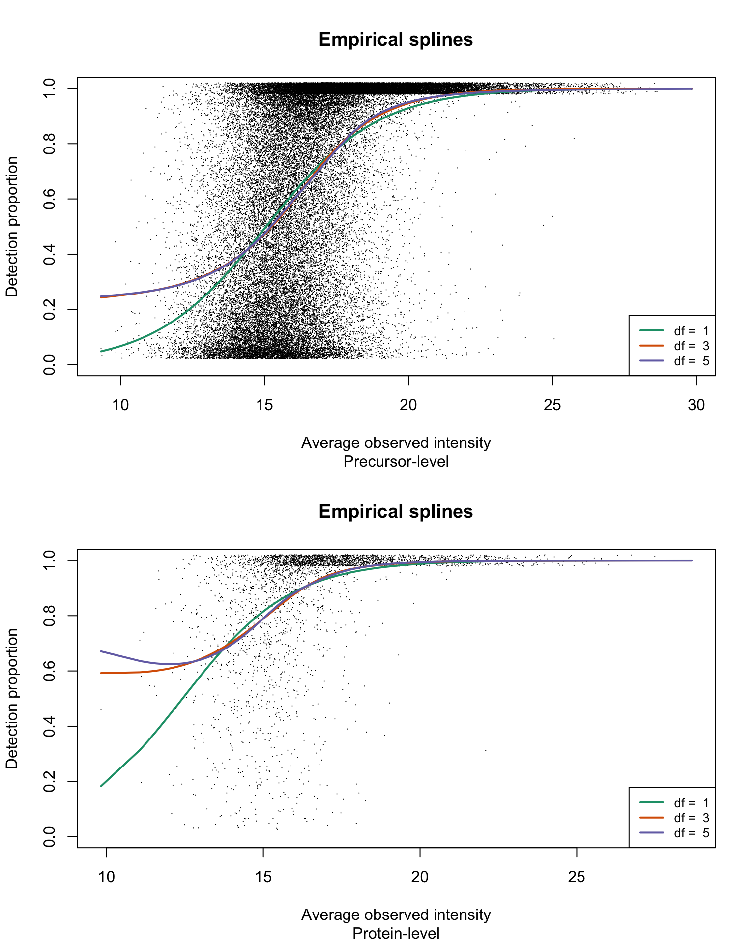
The analysis workflow presented in the manuscript is applied on the dataset on both precursor- and protein group-level data:

res <- list(prec = gatherResults(shbheart_prec), prot = gatherResults(shbheart_prot,
    b0.upper = Inf))

par(mfrow = c(2, 1))
for (res_i in 1:2) {
    eachRes <- res[[res_i]]
    for (i in 1:length(dfList)) {
        if (i == 1)
            plotEmpSplines(eachRes$nuis, X = eachRes$splineFits_params0[[i]]$X,
                eachRes$splineFits[[i]]$params, lineCol = lineColours[i],
                jitter.amount = 1/ncol(shbheart_prec)/2, point.cex = 0.15)
        if (i > 1)
            plotEmpSplines(eachRes$nuis, X = eachRes$splineFits_params0[[i]]$X,
                eachRes$splineFits[[i]]$params, lineCol = lineColours[i],
                newPlot = FALSE)
    }
    title(sub = c("Precursor-level", "Protein-level")[res_i])
    legend("bottomright", legend = paste("df = ", dfList), col = lineColours,
        lwd = 2, lty = 1, cex = 0.8)
}

Reduced deviance compared to an intercept model

devPlot1 <- ggplot(slice(res[[1]]$devs, 2:4), aes(x = df, y = percDevReduced)) +
    geom_point() + geom_line() + geom_text(aes(label = signif(percDevReduced,
    2)), vjust = -0.8) + scale_x_continuous(breaks = c(1, 3,
    5)) + labs(x = "d.f.", y = "Reduced deviance(%)") + ylim(0.9,
    1) + theme_classic() + ggtitle("Precursor-level")
devPlot2 <- ggplot(slice(res[[2]]$devs, 2:4), aes(x = df, y = percDevReduced)) +
    geom_point() + geom_line() + geom_text(aes(label = signif(percDevReduced,
    2)), vjust = -0.8) + scale_x_continuous(breaks = c(1, 3,
    5)) + labs(x = "d.f.", y = "Reduced deviance(%)") + ylim(0.9,
    1) + theme_classic() + ggtitle("Protein-level")
gridExtra::grid.arrange(devPlot1, devPlot2, ncol = 2)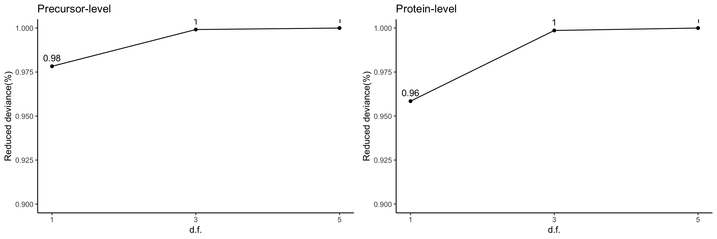

Empirical logit-linear curve with capped probabilities

par(mfrow = c(2, 1))
for (res_i in 1:2) {
    eachRes <- res[[res_i]]
    plotEmpSplines(eachRes$nuis, X = eachRes$splineFits_params0[[1]]$X,
        eachRes$cappedLinearFit$params, capped = TRUE, lineCol = lineColours[1],
        jitter.amount = 1/ncol(shbheart_prec)/2, point.cex = 0.15)
    title(sub = c("Precursor-level", "Protein-level")[res_i])
}

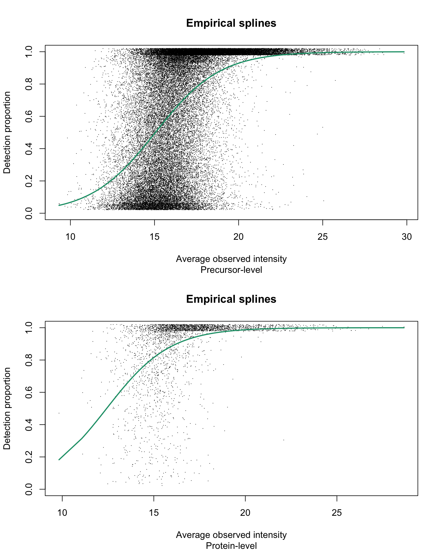
With estimated parameters on precursor-level data being:

round(res[["prec"]]$cappedLinearFit$params, 2)
alpha    b0    b1 
 1.00 -2.98 13.29

and estimated parameters on protein-level data being:

round(res[["prot"]]$cappedLinearFit$params, 2)
alpha    b0    b1 
 1.00 -1.50 13.55

Estimated \(\alpha\) values are equal to 1 on both precursor- and protein group-level data.

Detection probability curve assuming normal observed intensities

par(mfrow = c(2, 1))
for (res_i in 1:2) {
    eachRes <- res[[res_i]]
    plotDPC(eachRes$dpcFit, jitter.amount = 1/ncol(shbheart_prec)/2,
        point.cex = 0.15)
    title(sub = c("Precursor-level", "Protein-level")[res_i])
}

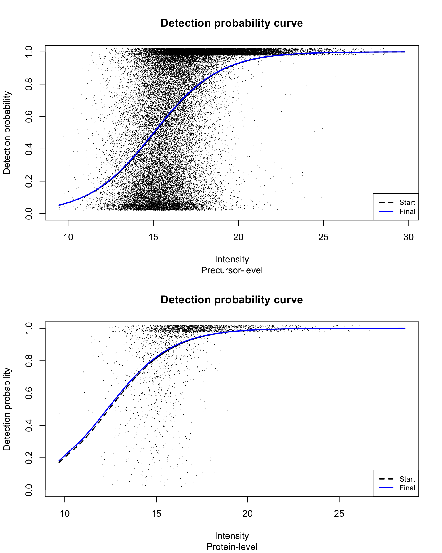
With estimated parameters on precursor-level data being:

round(res[["prec"]]$dpcFit$beta, 2)
   b0    b1 
-7.82  0.52

and estimated parameters on protein-level data being:

round(res[["prot"]]$dpcFit$beta, 2)
   b0    b1 
-7.04  0.57

Supplementary dataset: UPS1 spiked-in yeast extract

Three concentrations of UPS1 (25 fmol, 10 fmol and 5 fmol) were spiked in yeast extract (Giai Gianetto et al. 2016). This is a DDA dataset and MS raw data were processed by MaxQuant. Here we look at the dataset which compares 25 fmol to 10 fmol spiked-ins. Processed data were downloaded from ProteomeXchange Consortium via the PRIDE partner repository with the dataset identifier PXD002370. For peptide-level data, we use the peptides.txt file and for the protein-level analysis, we use the proteinGroups.txt file from the MaxQuant output. Log2-transformation is first applied before analysis.

Data summary

data("ratio2.5")
usp1_prec <- log2(ratio2.5$prec)
dim(usp1_prec)
[1] 13186     6
usp1_prot <- log2(ratio2.5$prot)
dim(usp1_prot)
[1] 2342    6

The overall proportion of missing data for the precursor-level data is

sum(is.na(usp1_prec))/length(usp1_prec)
[1] 0.147

The overall proportion of missing data for the protein-level data is

sum(is.na(usp1_prot))/length(usp1_prot)
[1] 0.06775

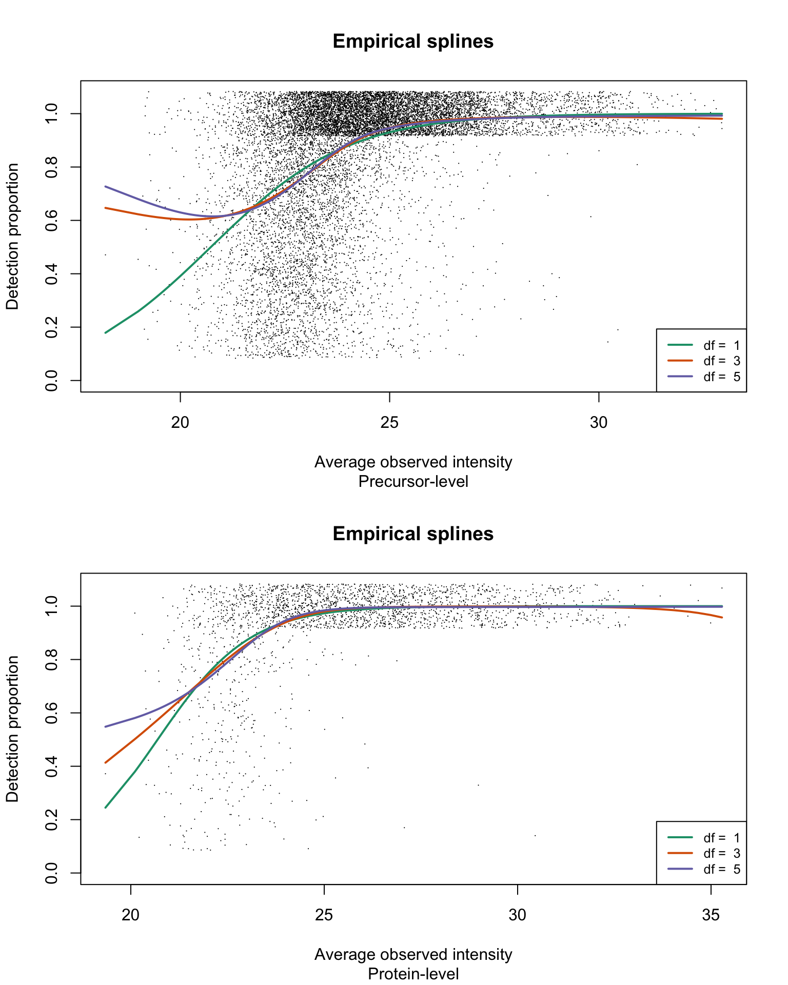
Empirical logistic splines for detected proportions

res <- list(prec = gatherResults(usp1_prec, b0.upper = Inf),
    prot = gatherResults(usp1_prot, b0.upper = Inf))

par(mfrow = c(2, 1))
for (res_i in 1:2) {
    eachRes <- res[[res_i]]
    for (i in 1:length(dfList)) {
        if (i == 1)
            plotEmpSplines(eachRes$nuis, X = eachRes$splineFits_params0[[i]]$X,
                eachRes$splineFits[[i]]$params, lineCol = lineColours[i],
                jitter.amount = 1/ncol(usp1_prec)/2, point.cex = 0.15,
                ylim = c(0, 1.08))
        if (i > 1)
            plotEmpSplines(eachRes$nuis, X = eachRes$splineFits_params0[[i]]$X,
                eachRes$splineFits[[i]]$params, lineCol = lineColours[i],
                newPlot = FALSE)
    }
    title(sub = c("Precursor-level", "Protein-level")[res_i])
    legend("bottomright", legend = paste("df = ", dfList), col = lineColours,
        lwd = 2, lty = 1, cex = 0.8)
}

Reduced deviance compared to an intercept model

devPlot1 <- ggplot(slice(res[[1]]$devs, 2:4), aes(x = df, y = percDevReduced)) +
    geom_point() + geom_line() + geom_text(aes(label = signif(percDevReduced,
    2)), vjust = -0.8) + scale_x_continuous(breaks = c(1, 3,
    5)) + labs(x = "d.f.", y = "Reduced deviance(%)") + ylim(0.9,
    1) + theme_classic() + ggtitle("Precursor-level")
devPlot2 <- ggplot(slice(res[[2]]$devs, 2:4), aes(x = df, y = percDevReduced)) +
    geom_point() + geom_line() + geom_text(aes(label = signif(percDevReduced,
    2)), vjust = -0.8) + scale_x_continuous(breaks = c(1, 3,
    5)) + labs(x = "d.f.", y = "Reduced deviance(%)") + ylim(0.9,
    1) + theme_classic() + ggtitle("Protein-level")
gridExtra::grid.arrange(devPlot1, devPlot2, ncol = 2)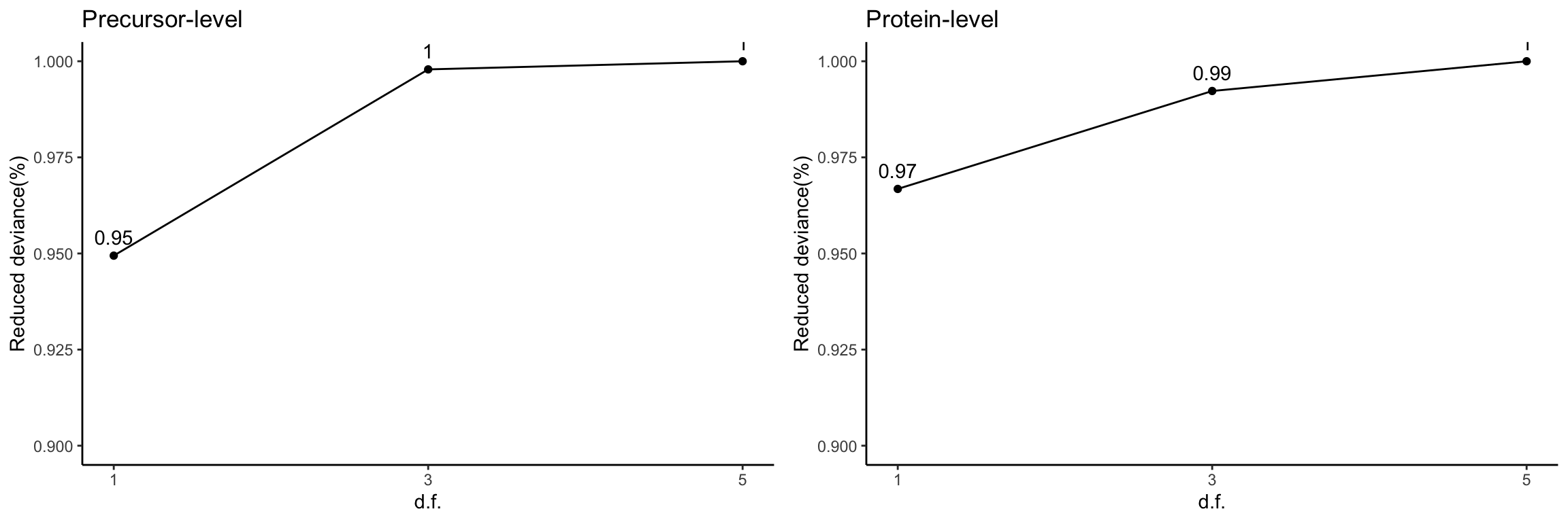

The spline with 1 degree of freedom contributes the majority to the total amount of reduced deviance in both precursor- and protein group-level data.

Empirical logit-linear curve with capped probabilities

par(mfrow = c(2, 1))
for (res_i in 1:2) {
    eachRes <- res[[res_i]]
    plotEmpSplines(eachRes$nuis, X = eachRes$splineFits_params0[[1]]$X,
        eachRes$cappedLinearFit$params, capped = TRUE, lineCol = lineColours[1],
        jitter.amount = 1/ncol(usp1_prec)/2, point.cex = 0.15,
        ylim = c(0, 1.08))
    title(sub = c("Precursor-level", "Protein-level")[res_i])
}

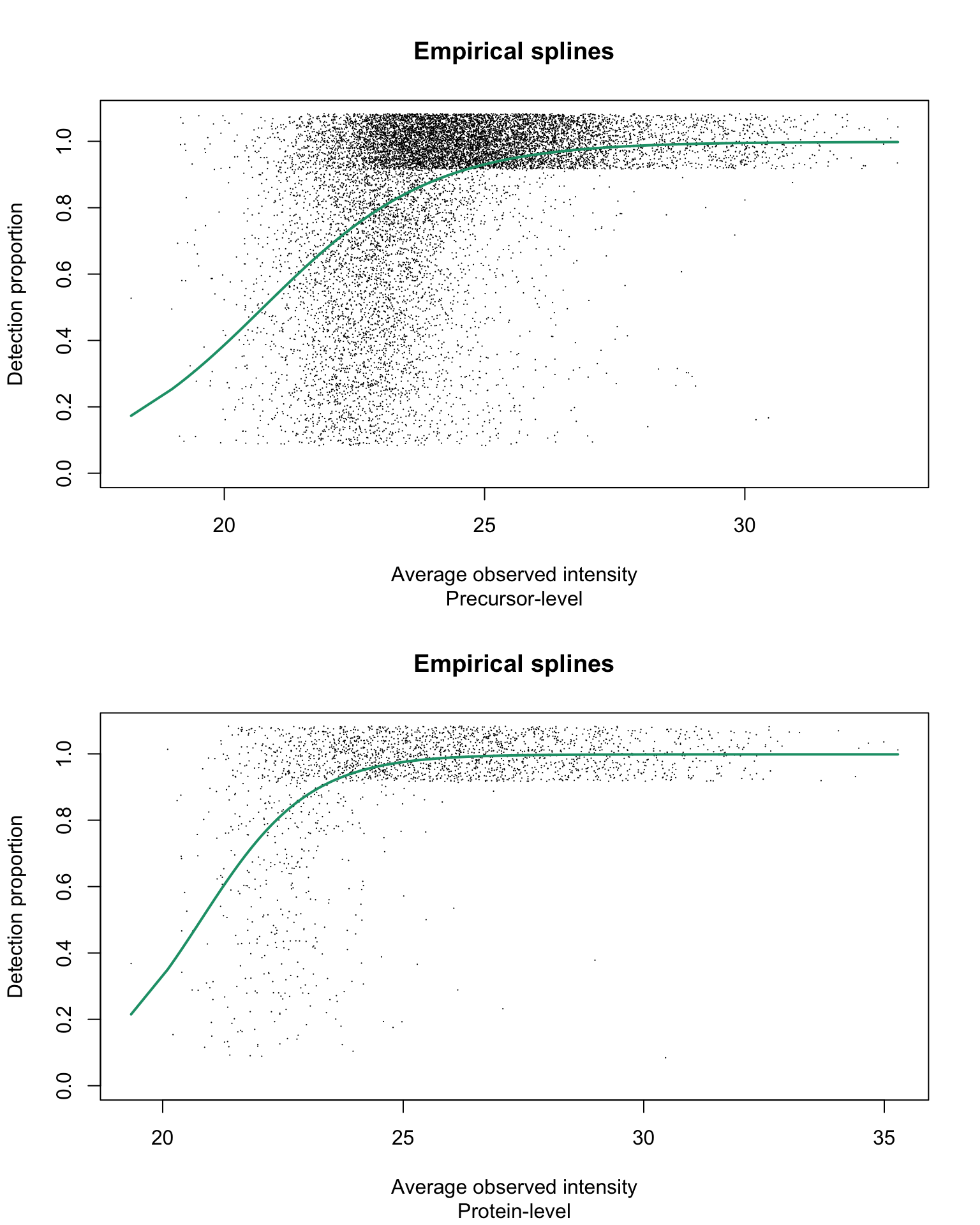
With estimated parameters on precursor-level data being:

round(res[["prec"]]$cappedLinearFit$params, 2)
alpha    b0    b1 
 1.00 -1.56 11.30

and estimated parameters on protein-level data being:

round(res[["prot"]]$cappedLinearFit$params, 2)
alpha    b0    b1 
 1.00 -1.29 17.70

Estimated \(\alpha\) values are 1 for both precursor- and protein group-level data.

Detection probability curve assuming normal observed intensities

par(mfrow = c(2, 1))
for (res_i in 1:2) {
    eachRes <- res[[res_i]]
    plotDPC(eachRes$dpcFit, jitter.amount = 1/ncol(usp1_prec)/2,
        point.cex = 0.15, ylim = c(0, 1.08))
    title(sub = c("Precursor-level", "Protein-level")[res_i])
}

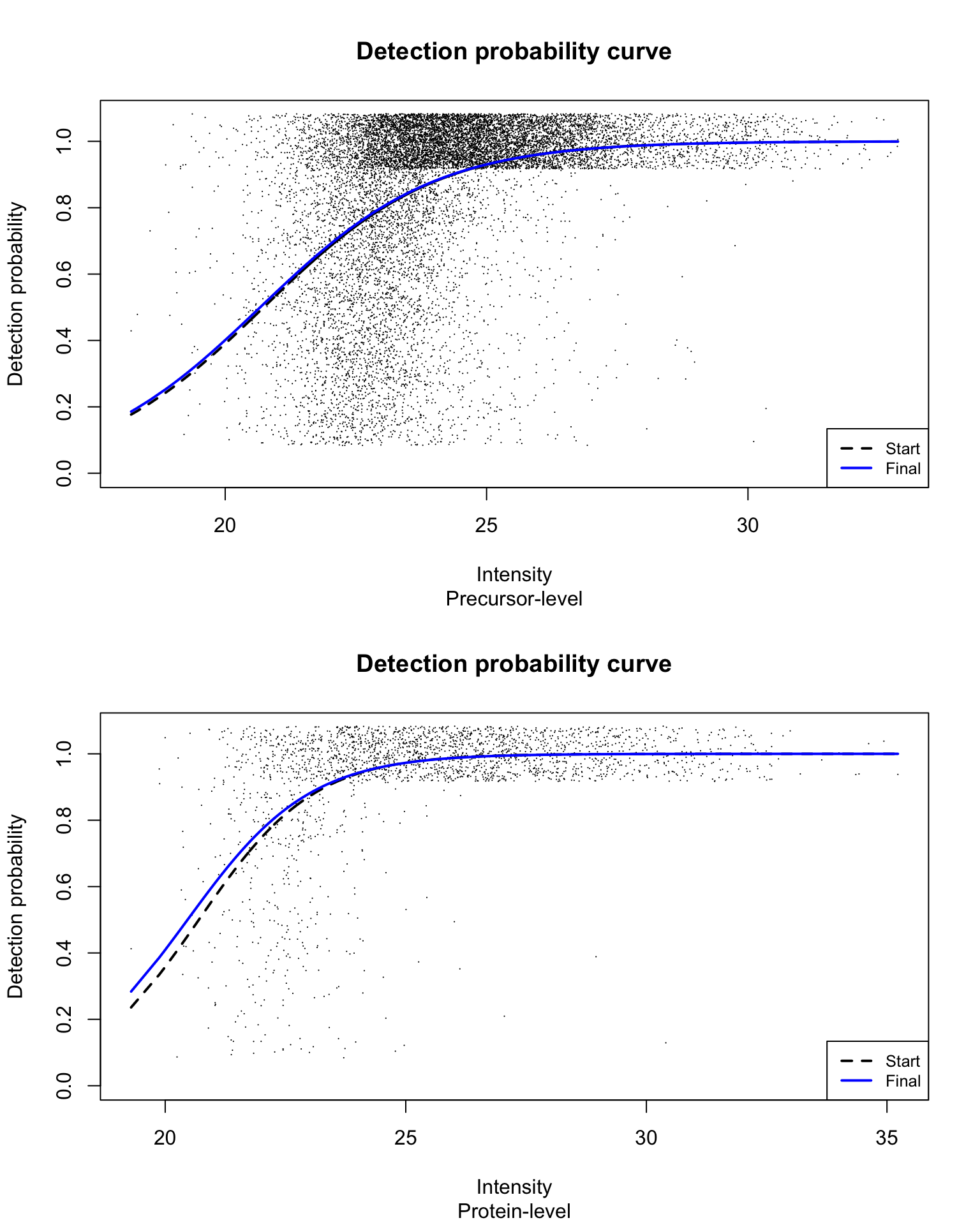
With estimated parameters for the fitted detection probability curve for precursor-level data being:

round(res$prec$dpcFit$beta, 2)
    b0     b1 
-12.38   0.60

and estimated parameters for the fitted detection probability curve for the protein group-level data being:

round(res$prot$dpcFit$beta, 2)
    b0     b1 
-16.16   0.79

References

Cox, Jürgen, Marco Y Hein, Christian A Luber, Igor Paron, Nagarjuna Nagaraj, and Matthias Mann. 2014. “Accurate Proteome-Wide Label-Free Quantification by Delayed Normalization and Maximal Peptide Ratio Extraction, Termed MaxLFQ.” Molecular & Cellular Proteomics 13 (9): 2513–26.

Demichev, Vadim, Christoph B Messner, Spyros I Vernardis, Kathryn S Lilley, and Markus Ralser. 2020. “DIA-NN: Neural Networks and Interference Correction Enable Deep Proteome Coverage in High Throughput.” Nature Methods 17 (1): 41–44.

Giai Gianetto, Quentin, Florence Combes, Claire Ramus, Christophe Bruley, Yohann Couté, and Thomas Burger. 2016. “Calibration Plot for Proteomics: A Graphical Tool to Visually Check the Assumptions Underlying FDR Control in Quantitative Experiments.” Proteomics 16 (1): 29–32.

Li, Mengbo, Benjamin L Parker, Evangeline Pearson, Benjamin Hunter, Jacob Cao, Yen Chin Koay, Oneka Guneratne, et al. 2020. “Core Functional Nodes and Sex-Specific Pathways in Human Ischaemic and Dilated Cardiomyopathy.” Nature Communications 11 (1): 1–12.

Session information

sessionInfo()
R version 4.3.1 (2023-06-16)
Platform: x86_64-apple-darwin20 (64-bit)
Running under: macOS Ventura 13.5.2

Matrix products: default
BLAS:   /Library/Frameworks/R.framework/Versions/4.3-x86_64/Resources/lib/libRblas.0.dylib 
LAPACK: /Library/Frameworks/R.framework/Versions/4.3-x86_64/Resources/lib/libRlapack.dylib;  LAPACK version 3.11.0

locale:
[1] en_US.UTF-8/en_US.UTF-8/en_US.UTF-8/C/en_US.UTF-8/en_US.UTF-8

time zone: Australia/Melbourne
tzcode source: internal

attached base packages:
[1] stats     graphics  grDevices utils     datasets  methods   base     

other attached packages:
 [1] protDP_1.1.0    lubridate_1.9.3 forcats_1.0.0   stringr_1.5.0   dplyr_1.1.3     purrr_1.0.2    
 [7] readr_2.1.4     tidyr_1.3.0     tibble_3.2.1    ggplot2_3.4.3   tidyverse_2.0.0

loaded via a namespace (and not attached):
 [1] sass_0.4.7         utf8_1.2.3         generics_0.1.3     stringi_1.7.12     hms_1.1.3         
 [6] digest_0.6.33      magrittr_2.0.3     RColorBrewer_1.1-3 timechange_0.2.0   evaluate_0.22     
[11] grid_4.3.1         fastmap_1.1.1      rprojroot_2.0.3    jsonlite_1.8.7     limma_3.57.9      
[16] gridExtra_2.3      formatR_1.14       fansi_1.0.5        scales_1.2.1       textshaping_0.3.7 
[21] jquerylib_0.1.4    cli_3.6.1          rlang_1.1.1        splines_4.3.1      munsell_0.5.0     
[26] withr_2.5.1        cachem_1.0.8       yaml_2.3.7         tools_4.3.1        tzdb_0.4.0        
[31] memoise_2.0.1      colorspace_2.1-0   vctrs_0.6.3        R6_2.5.1           lifecycle_1.0.3   
[36] fs_1.6.3           ragg_1.2.6         pkgconfig_2.0.3    desc_1.4.2         pkgdown_2.0.7     
[41] pillar_1.9.0       bslib_0.5.1        gtable_0.3.4       glue_1.6.2         statmod_1.5.0     
[46] systemfonts_1.0.5  xfun_0.40          tidyselect_1.2.0   rstudioapi_0.15.0  knitr_1.44        
[51] farver_2.1.1       htmltools_0.5.6.1  labeling_0.4.3     rmarkdown_2.25     compiler_4.3.1

Mengbo Li

Overview

Load packages

Dataset A: Hybrid proteome data

Data overview

Empirical logistic splines for detected proportions

Reduced deviance compared to an intercept model

Empirical logit-linear curve with capped probabilities

Detection probability curve assuming normal observed intensities

Dataset B: Cell cycle proteomes

Data overview

Empirical logistic splines for detected proportions

Reduced deviance compared to an intercept model

Empirical logit-linear curve with capped probabilities

Detection probability curve assuming normal observed intensities

Dataset C: HepG2 technical replicate data

Data overview

Empirical logistic splines for detected proportions

Reduced deviance compared to an intercept model

Empirical logit-linear curve with capped probabilities

Detection probability curve assuming normal observed intensities

Dataset D: Human blood plasma proteome

Data overview

Empirical logistic splines for detected proportions

Reduced deviance compared to an intercept model

Empirical logit-linear curve with capped probabilities

Detection probability curve assuming normal observed intensities

Supplementary dataset: Sydney heart bank data

Data summary

Empirical logistic splines for detected proportions

Reduced deviance compared to an intercept model

Empirical logit-linear curve with capped probabilities

Detection probability curve assuming normal observed intensities

Supplementary dataset: UPS1 spiked-in yeast extract

Data summary

Empirical logistic splines for detected proportions

Reduced deviance compared to an intercept model

Empirical logit-linear curve with capped probabilities

Detection probability curve assuming normal observed intensities

References

Session information